Inspect and plot Higher-Order Interactions

This example illustrates how to : 1. Inspect and analyse metric’s output 2. Plot Higher-Order Interactions

import matplotlib.pyplot as plt
import numpy as np
import xgi
from sklearn.preprocessing import MinMaxScaler

from hoi.metrics import InfoTopo
from hoi.plot import plot_landscape
from hoi.utils import get_nbest_mult

plt.style.use("ggplot")

Simulate data

In this first part, we simulate data to showcase how to analyse results

# create random data
np.random.seed(42)
x = np.random.rand(200, 6)

# inject redundancy between [0, 1, 2]
x[:, 0] += x[:, 1]
x[:, 2] += x[:, 1]

# inject synergy between [3, 4, 5]
x[:, 3] += x[:, 4] + x[:, 5]

Estimate HOI

The we can estimate the HOI. Here, we are going to use the InfoTopo metrics but you can use any implemented metric.

# define the model
model = InfoTopo(x)

# estimate hoi from order 3 up to order 6
hoi = model.fit(minsize=3, maxsize=6, method="gc")

  0%|          |  0/6 [00:00<?,       ?it/s]
 17%|█▋        | Entropy H(1):  1/6 [00:00<00:01,    4.78it/s]
 33%|███▎      | Entropy H(2):  2/6 [00:00<00:00,    4.72it/s]
 50%|█████     | Entropy H(3):  3/6 [00:00<00:00,    5.31it/s]
 67%|██████▋   | Entropy H(4):  4/6 [00:00<00:00,    5.97it/s]
 83%|████████▎ | Entropy H(5):  5/6 [00:00<00:00,    6.38it/s]
100%|██████████| Entropy H(6):  6/6 [00:00<00:00,    6.59it/s]


Mutual information:   0%|          | 0/42 [00:00<?, ?it/s]


Mutual information: 100%|██████████| 42/42 [00:00<00:00, 16093.62it/s]

Get a summary of the results

To get a summary table of the results, you can use the hoi.utils.get_nbest_mult() function. This functions returns a Pandas DataFrame with the highest and lowest values of hoi.

summary = get_nbest_mult(hoi, model=model)
print(summary)

   index  order       hoi     multiplet
0      0      3  0.196290     [0, 1, 2]
1     10      3  0.004351     [1, 2, 3]
2     13      3  0.004202     [1, 3, 4]
3     30      4  0.001593  [1, 2, 3, 4]
4      2      3  0.001399     [0, 1, 4]
5     27      4 -0.001132  [0, 2, 3, 5]
6     14      3 -0.001671     [1, 3, 5]
7      8      3 -0.001762     [0, 3, 5]
8     24      4 -0.002511  [0, 1, 3, 5]
9     19      3 -0.222631     [3, 4, 5]

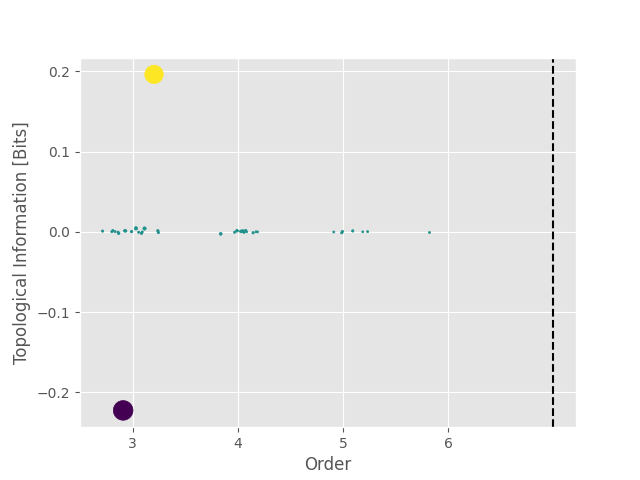
For the InfoTopo estimator, positive values of HOI refer to redundant interactions while negative values of HOI refer to synergistic interactions. As you can see from the summary table, we retrieve the multiplet [0, 1, 2] with the largest value and [3, 4, 5] with the smallest.

Landscape plot

The landscape plot can be used to visualize how the information spreads across orders. In our example, we only injected redundancy and synergy between triplets.

plot_landscape(hoi, model=model, kind="scatter")
plt.show()

Plotting individual multiplets

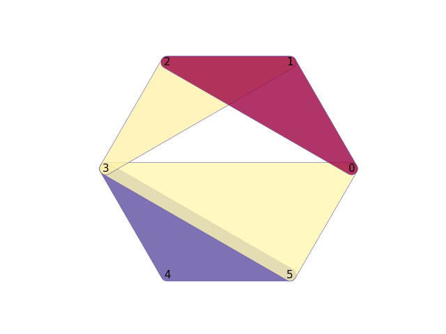
Alternatively, you can use the xgi Python package to plot individual multiplets. The example below the multiplets with the 2 highest redundancy and the two highest synergy.

# get summary
summary = get_nbest_mult(hoi, model=model, minsize=3, maxsize=3, n_best=2)

# extract the hoi values and the multiplets
hoi_order_3 = summary["hoi"]
mult_order_3 = summary["multiplet"]

# define an hypergraph object
H = xgi.Hypergraph()

# add the 6 nodes and define a circular layout
H.add_nodes_from(np.arange(6))
pos = xgi.drawing.layout.circular_layout(H)

# add edges
H.add_edges_from(mult_order_3.tolist())

# plot the hypergraph
ax, collections = xgi.draw(
    H,
    pos=pos,
    node_labels=True,
    font_size_nodes=11,
    node_size=0,
    edge_fc=hoi_order_3,
    edge_fc_cmap="Spectral_r",
    alpha=0.8,
    hull=True,
)
plt.show()

# sphinx_gallery_thumbnail_number = 2