Comparison of mutual-information estimators

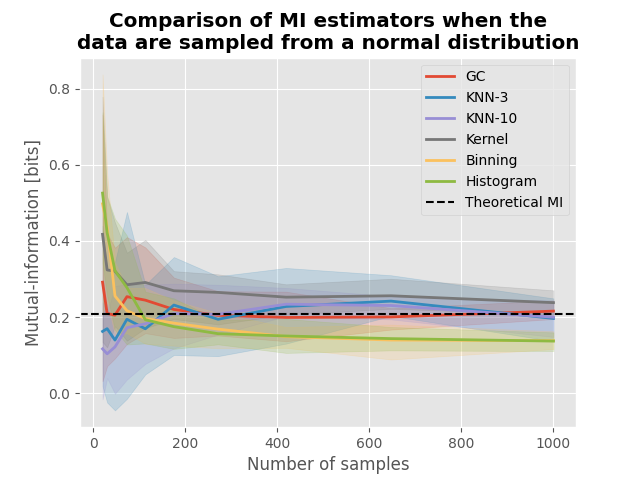
In this example, we are going to compare estimators of mutual-information (MI). In particular, the MI between variables sampled from a normal distribution can be estimated theoretically. In this this tutorial we are going to :

1. Simulate data sampled from a normal distribution

2. Define several estimators of MI

3. Compute the MI for a varying number of samples

4. See if the computed MI converge toward the theoretical value

import numpy as np
from functools import partial

from hoi.core import get_mi
from hoi.utils import digitize

import matplotlib.pyplot as plt

plt.style.use("ggplot")

Definition of MI estimators

Let us define several estimators of MI. We are going to use the GC MI (Gaussian Copula Mutual Information), the KNN (k Nearest Neighbor) and the kernel-based estimator, using the a binning approach and the histogram estimator. Please note that the histogram estimator is equivalent to the binning, with a correction that relate to the difference between the Shannon entropy of discrete variables and the differential entropy of continuous variables. This correction in the case of mutual information (MI) is not needed, because in the operation to compute the MI, the difference between discrete and differential entropy cancel out.

# create a special function for the binning approach as it requires binary data
mi_binning_fcn = get_mi("binning", base=2)


def mi_binning(x, y, **kwargs):
    x = digitize(x.T, **kwargs).T
    y = digitize(y.T, **kwargs).T

    return mi_binning_fcn(x, y)


# list of estimators to compare
metrics = {
    "GC": get_mi("gc", biascorrect=False),
    "KNN-3": get_mi("knn", k=3),
    "KNN-10": get_mi("knn", k=10),
    "Kernel": get_mi("kernel"),
    "Binning": partial(mi_binning, n_bins=4),
    "Histogram": get_mi("histogram", n_bins=4),
}

# number of samples to simulate data
n_samples = np.geomspace(20, 1000, 10).astype(int)

# number of repetitions to estimate the percentile interval
n_repeat = 10


# plotting function
def plot(mi, mi_theoric):
    """Plotting function."""
    for n_m, metric_name in enumerate(mi.keys()):
        # get the entropies
        x = mi[metric_name]

        # get the color
        color = f"C{n_m}"

        # estimate lower and upper bounds of the [5, 95]th percentile interval
        x_low, x_high = np.percentile(x, [5, 95], axis=0)

        # plot the MI as a function of the number of samples and interval
        plt.plot(n_samples, x.mean(0), color=color, lw=2, label=metric_name)
        plt.fill_between(n_samples, x_low, x_high, color=color, alpha=0.2)

    # plot the theoretical value
    plt.axhline(mi_theoric, linestyle="--", color="k", label="Theoretical MI")
    plt.legend()
    plt.xlabel("Number of samples")
    plt.ylabel("Mutual-information [bits]")

MI of data sampled from normal distribution

Given two variables \(X \sim \mathcal{N}(\mu_{x}, \sigma_{x})\) and \(Y \sim \mathcal{N}(\mu_{y}, \sigma_{y})\), linked by a covariance \(\sigma_{xy}\) the theoretical MI in bits is defined by :

\[I(X; Y) = \frac{1}{2} \times log_{2}(\frac{\sigma_{x}^{2}\sigma_{y}^{2}}{ \sigma_{x}^{2}\sigma_{y}^{2} - \sigma_{xy}^{2} })\]

# mean and standard error of x and y variables
mu_x = 0.0
mu_y = 0.0
sigma_x = 1.0
sigma_y = 1.0

# covariance between x and y
covariance = 0.5

# covariance matrix
cov_matrix = [[sigma_x**2, covariance], [covariance, sigma_y**2]]

# define the theoretic MI
mi_theoric = 0.5 * np.log2(
    sigma_x**2 * sigma_y**2 / (sigma_x**2 * sigma_y**2 - covariance**2)
)

# compute mi using various metrics
mi = {k: np.zeros((n_repeat, len(n_samples))) for k in metrics.keys()}

for n_s, s in enumerate(n_samples):
    for n_r in range(n_repeat):
        for metric, fcn in metrics.items():
            # generate samples from joint gaussian distribution
            fx = np.random.multivariate_normal([mu_x, mu_y], cov_matrix, s)

            # extract x and y
            x = fx[:, [0]].T
            y = fx[:, [1]].T

            # compute mi
            mi[metric][n_r, n_s] = fcn(x, y)

# plot the results
plot(mi, mi_theoric)
plt.title(
    "Comparison of MI estimators when the\ndata are sampled from a "
    "normal distribution",
    fontweight="bold",
)
plt.show()