Comparison of entropy estimators for a multivariate normal

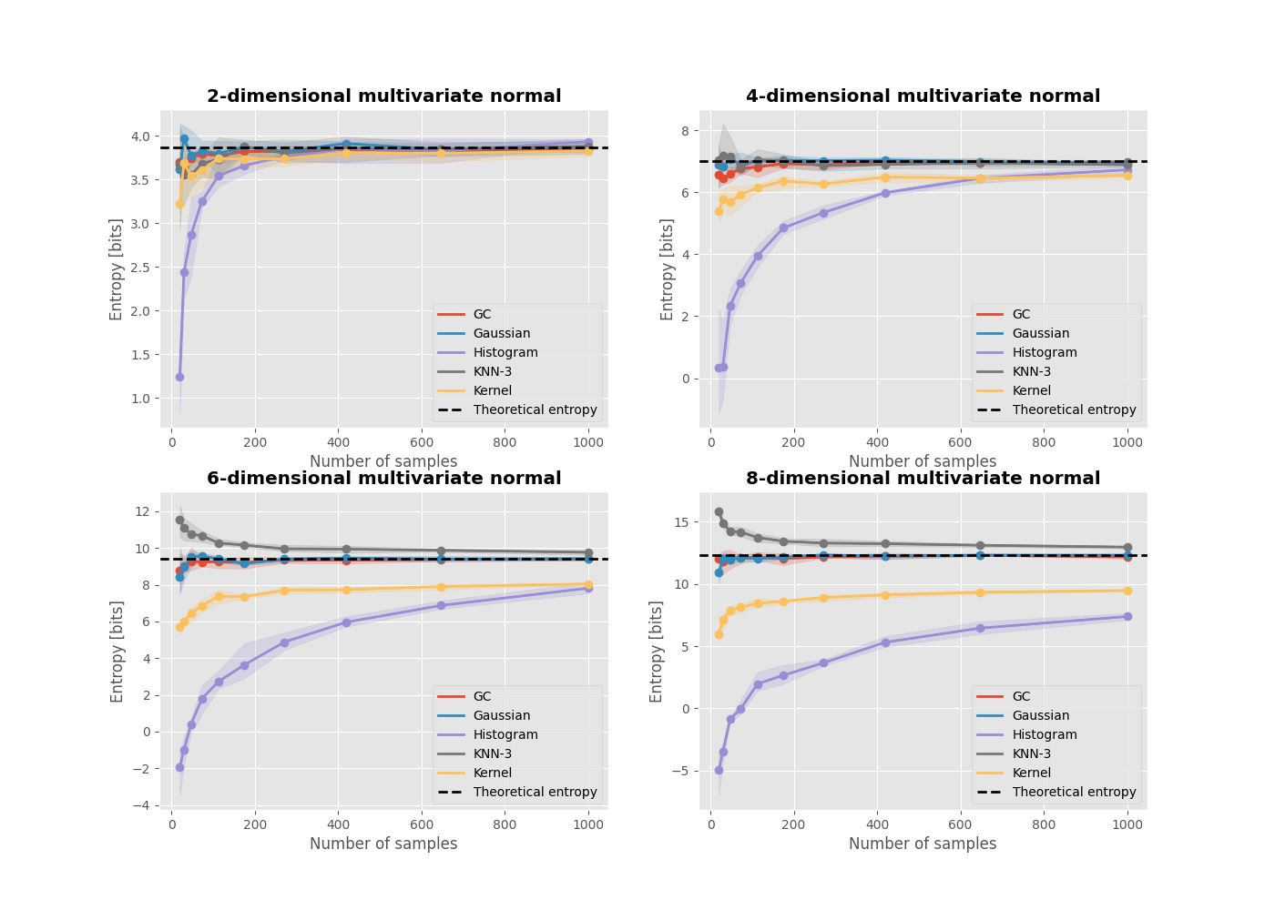
When calculating Higher-Order Interactions using entropy-based metrics, the process includes estimating the entropy of multivariate variables. Nevertheless, certain entropy estimators may not function optimally as the number of dimensions increases. This can be demonstrated through an example where various entropy estimators are compared using data sampled from a multivariate normal distribution with increasing dimensionality.

import numpy as np

from sklearn.datasets import make_spd_matrix

from hoi.core import get_entropy

import matplotlib.pyplot as plt

plt.style.use("ggplot")

Definition of estimators of entropy

Let us define several estimators of entropy. We are going to use the GC (Gaussian Copula), the KNN (k Nearest Neighbor), the kernel-based, the Gaussian estimators and the histogram estimator.

# list of estimators to compare
metrics = {
    "GC": get_entropy("gc"),
    "Gaussian": get_entropy("gauss"),
    "Histogram": get_entropy("histogram"),
    "KNN-3": get_entropy("knn", k=3),
    "Kernel": get_entropy("kernel"),
}

# number of samples to simulate data
n_samples = np.geomspace(20, 1000, 10).astype(int)

# number of repetitions to estimate the percentile interval
n_repeat = 5

Now we define the plotting function. This function plot the entropy as a function of sample size, for each estimator. It also plots the theoretical entropy with an horizontal dotted black line.

# plotting function
def plot(h_x, h_theoric, n):
    """Plotting function."""
    for n_m, metric_name in enumerate(h_x.keys()):
        # get the entropies
        x = h_x[metric_name]

        # get the color
        color = f"C{n_m}"

        # estimate lower and upper bounds of the [5, 95]th percentile interval
        x_low, x_high = np.percentile(x, [5, 95], axis=0)

        # plot the entropy as a function of the number of samples and interval
        plt.plot(n_samples, x.mean(0), color=color, lw=2, label=metric_name)
        plt.plot(n_samples, x.mean(0), color=color, marker="o")
        plt.fill_between(n_samples, x_low, x_high, color=color, alpha=0.2)

    # plot the theoretical value
    plt.axhline(
        h_theoric, linestyle="--", color="k", label="Theoretical entropy", lw=2
    )
    plt.legend()
    plt.xlabel("Number of samples")
    plt.ylabel("Entropy [bits]")
    plt.title(f"{n}-dimensional multivariate normal", fontweight="bold")

Then we create a function to generate a covariance matrix that is then going to be used for simulating the multivariate normal. The function below takes a single input describing the dimensionality of the multivariate normal.

def get_covariance(n):
    """Get a symmetric positive semi-definite covariance matrix."""
    # random covariance matrix
    cov = make_spd_matrix(n)

    # Normalize the covariance matrix to have diagonal elements equal to one
    d = np.sqrt(np.diag(cov))
    cov = cov / d[:, None]
    cov = cov / d[None, :]

    # compute theoretic entropy
    h = (0.5 * np.log((2 * np.pi * np.e) ** n * np.linalg.det(cov))) / np.log(
        2
    )

    return cov, h

Finally, we also create a function to compute the entropies, using the defined estimators for an increasing sample size.

def compute_entropies(cov):
    # compute entropies using various metrics
    h_x = {k: np.zeros((n_repeat, len(n_samples))) for k in metrics.keys()}

    for metric, fcn in metrics.items():
        for n_s, s in enumerate(n_samples):
            for n_r in range(n_repeat):
                x = np.random.multivariate_normal(
                    [0] * cov.shape[0], cov, size=(s)
                ).T
                h_x[metric][n_r, n_s] = fcn(x)

    return h_x

Comparison of estimators

Now we can make the final figure. Each subplot contains the comparison between estimators for a n-dimensional multivariate normal. For such distribution, the theoretical entropy is defined as :

\[H(X) = \frac{1}{2} \times log((2πe)^{n} |\Sigma|) / log(2)\]

with e the Euler constant, \(|\Sigma|\) the determinant of the covariance matrix and n the dimensionality of the multivariate normal.

fig, axs = plt.subplots(2, 2, figsize=(14, 10))

plt.sca(axs[0, 0])
n = 2
cov, h_theoric = get_covariance(n)
h_x = compute_entropies(cov)
plot(h_x, h_theoric, n)

plt.sca(axs[0, 1])
n = 4
cov, h_theoric = get_covariance(n)
h_x = compute_entropies(cov)
plot(h_x, h_theoric, n)

plt.sca(axs[1, 0])
n = 6
cov, h_theoric = get_covariance(n)
h_x = compute_entropies(cov)
plot(h_x, h_theoric, n)

plt.sca(axs[1, 1])
n = 8
cov, h_theoric = get_covariance(n)
h_x = compute_entropies(cov)
plot(h_x, h_theoric, n)

plt.show()