Comparison of MI estimators with high-dimensional data

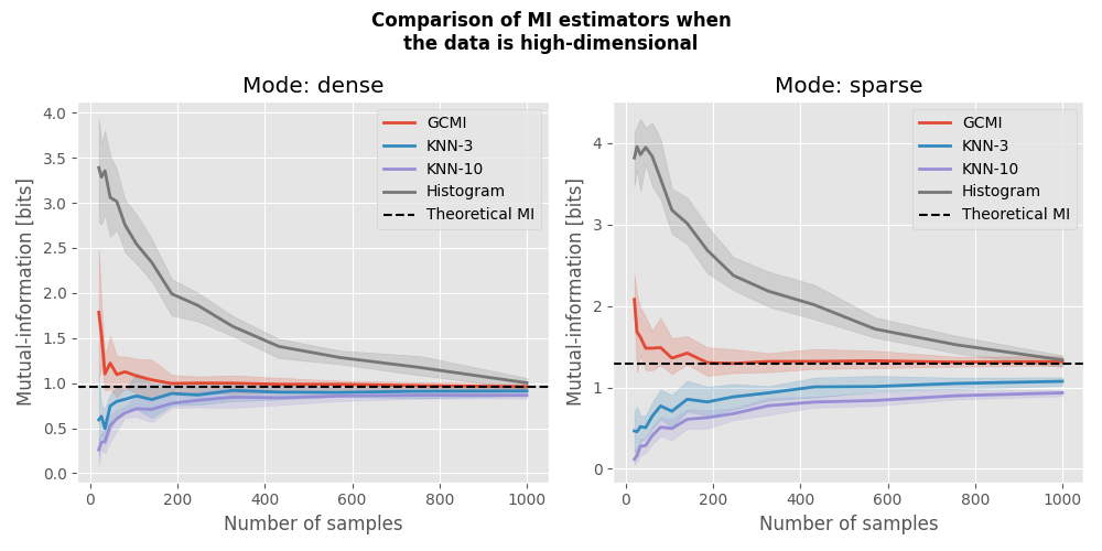
In this example, we are going to compare estimators of mutual-information (MI) with high-dimensional data. In particular, the MI between variables sampled from a multinormal distribution can be estimated theoretically. In this this tutorial we are going to:

1. Simulate data sampled from a “splitted” multivariate normal distribution.

2. Define estimators of MI.

3. Compute the MI for a varying number of samples.

4. See if the computed MI converge towards the theoretical value.

This example is inspired from a similar simulation done by Czyz et al., NeurIPS 2023 [6].

import numpy as np

from hoi.core import get_mi

import matplotlib.pyplot as plt

plt.style.use("ggplot")

Definition of MI estimators

We are going to use the GCMI (Gaussian Copula Mutual Information), KNN (k Nearest Neighbor) and histogram estimator.

# list of estimators to compare
metrics = {
    "GCMI": get_mi("gc", biascorrect=False),
    "KNN-3": get_mi("knn", k=3),
    "KNN-10": get_mi("knn", k=10),
    "Histogram": get_mi("histogram", n_bins=3),
}

# number of samples to simulate data
n_samples = np.geomspace(20, 1000, 15).astype(int)

# number of repetitions to estimate the percentile interval
n_repeat = 10


# plotting function
def plot(mi, mi_theoric, ax):
    """Plotting function."""
    for n_m, metric_name in enumerate(mi.keys()):
        # get the entropies
        x = mi[metric_name]

        # get the color
        color = f"C{n_m}"

        # estimate lower and upper bounds of the [5, 95]th percentile interval
        x_low, x_high = np.percentile(x, [5, 95], axis=0)

        # plot the MI as a function of the number of samples and interval
        ax.plot(n_samples, x.mean(0), color=color, lw=2, label=metric_name)
        ax.fill_between(n_samples, x_low, x_high, color=color, alpha=0.2)

    # plot the theoretical value
    ax.axhline(mi_theoric, linestyle="--", color="k", label="Theoretical MI")
    ax.legend()
    ax.set_xlabel("Number of samples")
    ax.set_ylabel("Mutual-information [bits]")

MI of data sampled from splitted multinormal distribution

Given two variables \(X \sim \mathcal{N}(\vec{\mu_{x}}, \Sigma_{x})\) and \(Y \sim \mathcal{N}(\vec{\mu_{y}}, \Sigma_{y})\), linked by a covariance \(C\) the theoretical MI in bits is defined by :

\[I(X; Y) = \frac{1}{2} \times log_{2}(\frac{|\Sigma_{x}||\Sigma_{y}|}{|\Sigma|})\]

# function for creating the covariance matrix with differnt modes
def create_cov_matrix(n_dims, cov, mode="dense", k=None):
    """Create a covariance matrix."""
    # variance of x and y, for each dimension, 1
    cov_matrix = np.eye(2 * n_dims)
    if mode == "dense":
        # all dimensions, but diagonal, with covariance cov
        cov_matrix += cov
        cov_matrix[np.diag_indices(2 * n_dims)] = 1
    elif mode == "sparse":
        # only pairs xi, yi with i < k have covariance cov
        k = k if k is not None else n_dims
        for i in range(n_dims):
            if i < k:
                cov_matrix[i, i + n_dims] = cov
                cov_matrix[i + n_dims, i] = cov

    return cov_matrix


def compute_true_mi(cov_matrix):
    """Compute the true MI (bits)."""
    n_dims = cov_matrix.shape[0] // 2
    det_x = np.linalg.det(cov_matrix[n_dims:, n_dims:])
    det_y = np.linalg.det(cov_matrix[:n_dims, :n_dims])
    det_xy = np.linalg.det(cov_matrix)
    return 0.5 * np.log2(det_x * det_y / det_xy)


# number of dimensions per variable
n_dims = 4
# mean
mu = [0.0] * n_dims * 2
# covariance
covariance = 0.6

# modes for the covariance matrix:
# - dense: off diagonal elements have specified covariance
# - sparse: only pairs xi, yi with i < k have specified covariance
modes = ["dense", "sparse"]
# number of pairs with specified covariance
k = n_dims

fig = plt.figure(figsize=(10, 5))
# compute mi using various metrics
mi = {k: np.zeros((n_repeat, len(n_samples))) for k in metrics.keys()}
for i, mode in enumerate(modes):
    cov_matrix = create_cov_matrix(n_dims, covariance, mode=mode)
    # define the theoretic MI
    mi_theoric = compute_true_mi(cov_matrix)
    ax = fig.add_subplot(1, 2, i + 1)

    for n_s, s in enumerate(n_samples):
        for n_r in range(n_repeat):
            # generate samples from joint gaussian distribution
            fx = np.random.multivariate_normal(mu, cov_matrix, s)
            for metric, fcn in metrics.items():
                # extract x and y
                x = fx[:, :n_dims].T
                y = fx[:, n_dims:].T
                # compute mi
                mi[metric][n_r, n_s] = fcn(x, y)

    # plot the results
    plot(mi, mi_theoric, ax)
    ax.title.set_text(f"Mode: {mode}")

fig.suptitle(
    "Comparison of MI estimators when\nthe data is high-dimensional",
    fontweight="bold",
)
fig.tight_layout()
plt.show()