Machine-learning vs. Information theoretic approaches for HOI

This example compares Machine-learning and Information theoretic approaches to investigate Higher Order Interactions.

import numpy as np

from sklearn.discriminant_analysis import LinearDiscriminantAnalysis
from sklearn.model_selection import cross_val_score

from hoi.metrics import GradientOinfo

import matplotlib.pyplot as plt
plt.style.use('ggplot')

Data simulation

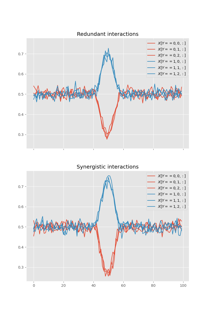
Let’s start by creating a function that simulates higher-order interactions between a multivariate variable \(X={X_{1}, ..., X_{N}}\) and a univariate variable \(Y\). We are then going to create redundant and synergistic relationships between \(X\) and \(Y\). To introduce redundancy between the two, each \(X_{i}\) is going to receive a copy of \(Y\). To create synergy, each \(X_{i}\) is going to encode different parts of \(Y\) so that \(Y\) can only be fully known when all the \(X_{i}\) are provided. For further information about how to simulate redundant and synergistic interactions, checkout the example How to simulate redundancy and synergy

def simulate_data(
    n_samples=300,
    n_x=3,
    n_times=100,
    t_start=40,
    t_end=60,
    rel_type="redundancy",
    rel_strength=0.2,
):
    """Data simulation.

    Parameters
    ----------
    n_samples : int, 300
        Number of samples in x and y
    n_x : int, 3
        Number of features in x
    n_times : int, 100
        Number of time points in x
    t_start : int, 40
        Time sample at which the relation between x and y starts
    t_end : int, 60
        Time sample at which the relation between x and y ends
    rel_type : {"redundancy", "synergy"}
        Specify whether the nature of the relationship between x and y. Use
        either "redundancy" or "synergy"
    rel_strength : float, 0.2
        Strength of the statistical dependency between x and y

    Returns
    -------
    x : array_like
        Array of shape (n_samples, n_x, n_times)
    y : array_like
        Target array of shape (n_samples)
    """
    assert rel_type in ["redundancy", "synergy"]

    sl = slice(t_start, t_end)
    hann = np.hanning(t_end - t_start)
    y = np.random.permutation([0] * n_samples + [1] * n_samples)
    y_norm = 2 * y - 1

    if rel_type == "redundancy":
        x = np.random.rand(2 * n_samples, n_x, n_times)
        x[..., sl] += (
            rel_strength * y_norm.reshape(-1, 1, 1) * hann.reshape(1, 1, -1)
        )
    elif rel_type == "synergy":
        x = np.random.rand(2 * n_samples, n_x, n_times)
        trial_blocks = np.array_split(np.arange(n_samples * 2), n_x)
        for n_r in range(n_x):
            _trials = trial_blocks[n_r]
            x[_trials, n_r, sl] += (
                rel_strength
                * y_norm[_trials].reshape(-1, 1)
                * hann.reshape(1, -1)
            )

    return x, y

Now we can create two pairs of variables \((X_{red}, Y_{red})\) and \((X_{syn}, Y_{syn})\) with respectively redundant and synergistic relationships between them

x_red, y_red = simulate_data(rel_type="redundancy", rel_strength=0.2)
x_syn, y_syn = simulate_data(rel_type="synergy", rel_strength=0.7)

Let’s plot the data

def plot_xy(x, y):
    for n_y, u in enumerate(np.unique(y)):
        for n_x in range(x.shape[1]):
            u_x = x[y == u, n_x, :]
            x_m = u_x.mean(0)
            plt.plot(x_m, color=f"C{n_y}", label=rf"$X[Y == {u}, {n_x}, :]$")
    plt.legend()

fig, axs = plt.subplots(2, 1, figsize=(8, 12), sharex=True, sharey=True)
axs = np.ravel(axs)
plt.sca(axs[0])
plot_xy(x_red, y_red)
plt.title("Redundant interactions")
plt.sca(axs[1])
plot_xy(x_syn, y_syn)
plt.title("Synergistic interactions")
plt.show()

Decoding Y using X

Now let’s try to decode the \(Y\) variable using \(X\).

def decode_y(x, y):
    clf = LinearDiscriminantAnalysis()
    _, n_x, n_times = x.shape
    da = np.zeros((n_x + 1, n_times))
    for t in range(n_times):
        for n_r in range(n_x):
            da[n_r, t] = cross_val_score(clf, x[:, n_r, [t]], y, cv=5).mean()
        da[-1, t] = cross_val_score(clf, x[:, :, t], y, cv=5).mean()

    return 100 * da


def plot_decoding(da):
    for k in range(da.shape[0] - 1):
        plt.plot(da[k, :], color="k", label=r"$DA_{X_{%i}}$" % (k + 1))
    plt.plot(da[-1, :], color="C0", label=r"$DA_{X_{1}, ..., X_{N}}$", lw=4)
    plt.legend()

fig, axs = plt.subplots(2, 1, figsize=(8, 12), sharex=True, sharey=True)
axs = np.ravel(axs)
plt.sca(axs[0])
plot_decoding(decode_y(x_red, y_red))
plt.ylabel("Decoding accuracy [%]")
plt.title("Redundant interactions", fontweight="bold")
plt.sca(axs[1])
plot_decoding(decode_y(x_syn, y_syn))
plt.ylabel("Decoding accuracy [%]")
plt.title("Synergistic interactions", fontweight="bold")
plt.show()

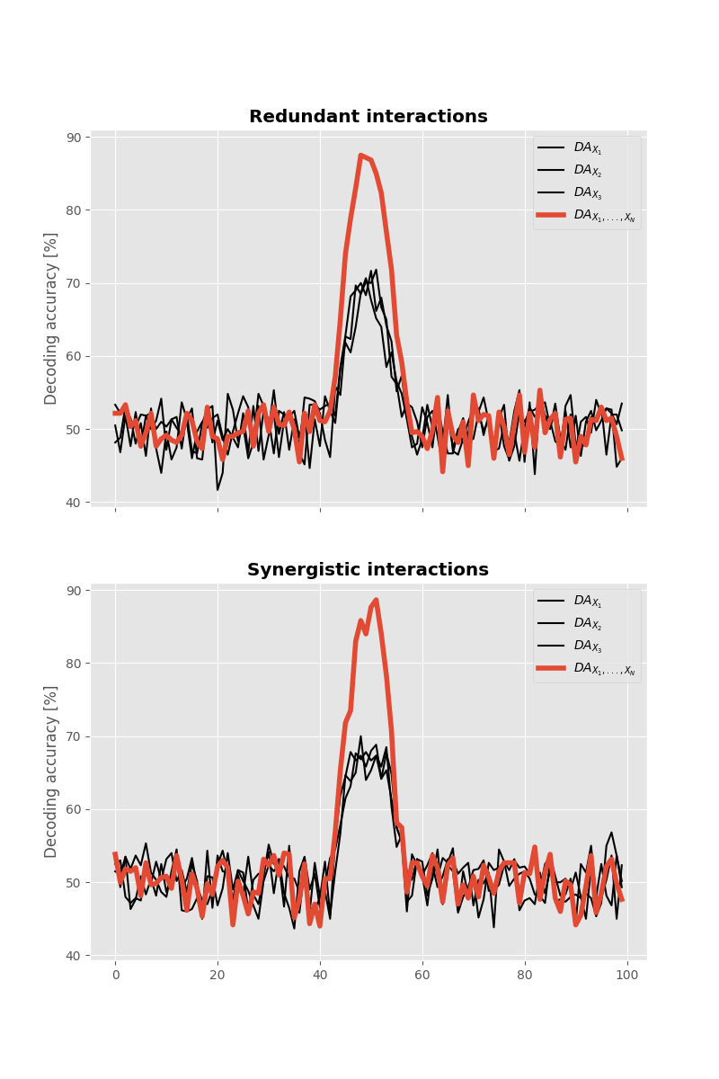
As we can see, using machine-learning we can decode the \(Y\) variable with a decoding accuracy of ~90% when there’s either redundant or synergistic interactions between \(X\) and \(Y\)

Using information-theoretic approaches

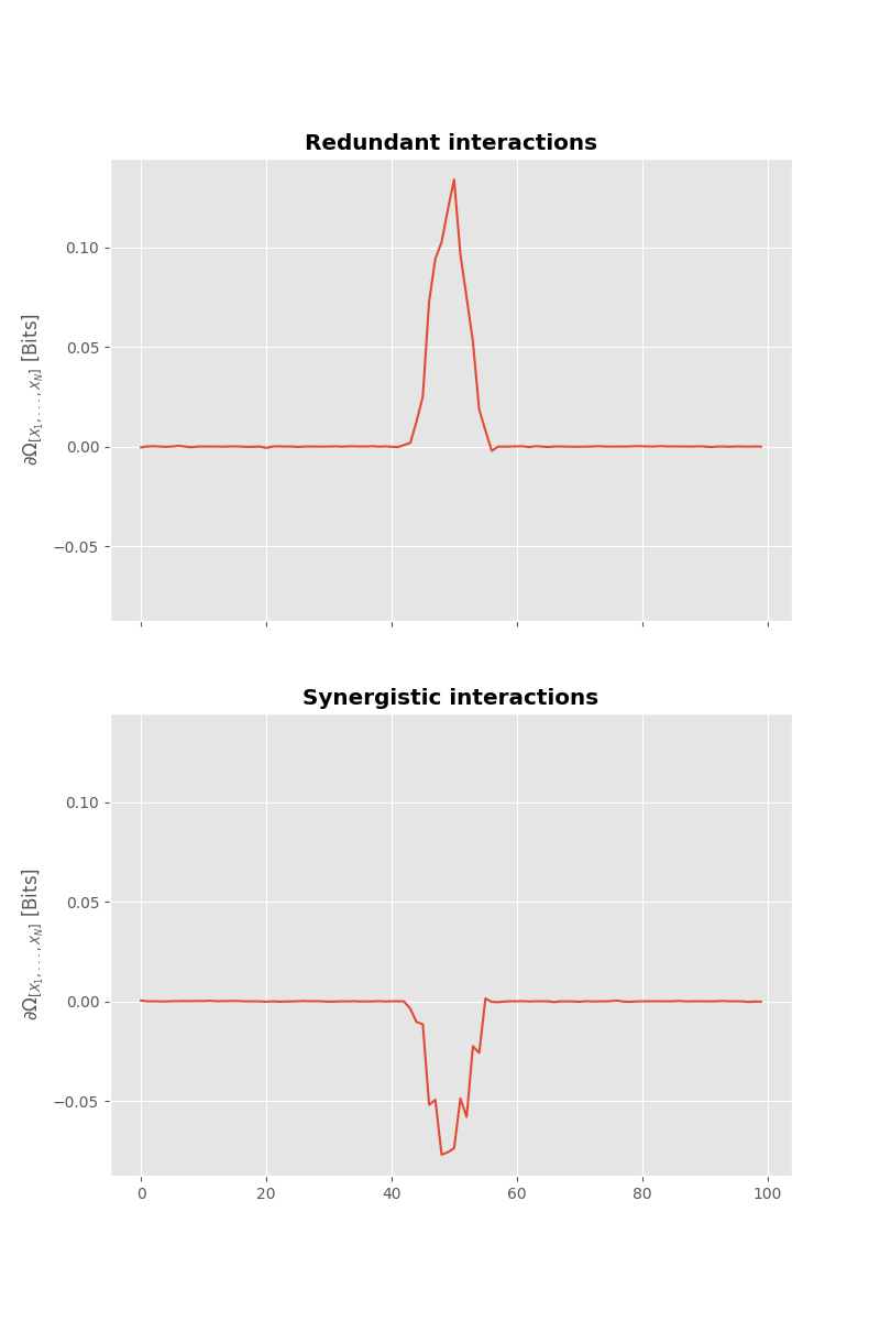
Now let’s information-theoretic approaches. The question we try to answer here is whether the \(X_{i}\) are carrying redundant or synergistic information about \(Y\). To answer this question we are going to use the Gradient Oinfo.

def it(x, y):
    model = GradientOinfo(x, y, verbose=False)
    return model.fit(minsize=3, maxsize=3)


fig, axs = plt.subplots(2, 1, figsize=(8, 12), sharex=True, sharey=True)
axs = np.ravel(axs)
plt.sca(axs[0])
plt.plot(it(x_red, y_red).squeeze())
plt.ylabel(r"$\partial \Omega_{[X_{1}, ..., X_{N}]}$ [Bits]")
plt.title("Redundant interactions", fontweight="bold")
plt.sca(axs[1])
plt.plot(it(x_syn, y_syn).squeeze())
plt.ylabel(r"$\partial \Omega_{[X_{1}, ..., X_{N}]}$ [Bits]")
plt.title("Synergistic interactions", fontweight="bold")
plt.show()

We retrieve the bump of information around sample 50 however this time, the bump is positive in case of redundant interactions and negative in case of synergistic interactions.