How to simulate redundancy and synergy

How to simulate redundancy and synergy#

Redundancy and Synergy are terms defining how variables are interacting. In this tutorial, we are going to see simple and intuitive ways of simulating redundancy and synergy in two different context :

Network behavior : i.e. redundant and synergistic interactions between elements (or nodes) of a network
Network encoding : i.e. nodes of a network engaged in redundant and synergistic interactions about a target variable.

import numpy as np

from hoi.metrics import Oinfo, GradientOinfo
from hoi.simulation import simulate_hoi_gauss

import matplotlib.pyplot as plt

np.random.seed(42)
plt.style.use("ggplot")

Redundant and synergistic network behavior#

In this first part, we are going to create a multivariate gaussian variable X with specific information patterns. Then we need a function to estimate whether the interactions between the three nodes are more redundant or more synergistic. To estimate whether the interactions between the three nodes are redundant or synergistic, we are going to use the hoi.metrics.Oinfo. When the Oinfo is positive, it means that the interactions are redundant and if the Oinfo is negative, the interactions are synergistic.

# function to estimate the nature of the interactions
def compute_hoi_beh(x):
    """This function computes the HOI using the Oinfo."""
    model = Oinfo(x)
    hoi = model.fit(method="gc", minsize=3, maxsize=3)
    return hoi.squeeze()

Simulating synergistic behavior#

In gaussian multivariate data, it is possible to generate synergy and redundancy by setting the parameters of the covariance matrix. This can be done using the function hoi.simulation.simulate_hoi_gauss, in the following way:

# x = (n_samples, n_nodes)
x = simulate_hoi_gauss(
    target=False, n_samples=1000, triplet_character="synergy"
)

compute hoi using the Oinfo

hoi = compute_hoi_beh(x)

  0%|          |  0/1 [00:00<?,       ?it/s]
100%|██████████| Oinfo (3):  1/1 [00:00<00:00,    1.56it/s]

Print HOI value

print(f"HOI between nodes (1, 2, 3) : {hoi}")

HOI between nodes (1, 2, 3) : -0.8529834747314453

As we can see, the estimated HOI is negative which is the hallmark of synergy when using the Oinfo. Be careful because some metrics are positive for synergistic interactions.

Simulating redundant behavior#

As for the redundancy, we can generate three gaussian variables, presenting redundant behavior, using the function, hoi.simulation.simulate_hoi_gauss, in the following way:

# x = (n_samples, n_nodes)
x = simulate_hoi_gauss(
    target=False, n_samples=1000, triplet_character="redundancy"
)

compute hoi using the Oinfo

hoi = compute_hoi_beh(x)

  0%|          |  0/1 [00:00<?,       ?it/s]
100%|██████████| Oinfo (3):  1/1 [00:00<00:00,    6.07it/s]

Print HOI value

print(f"HOI between nodes (1, 2, 3) : {hoi}")

HOI between nodes (1, 2, 3) : 0.28618431091308594

Now HOI is positive, therefore the interaction between the three nodes is dominated by redundancy.

Simulating synergistic behavior by sum operation#

A synergy is obtained when elements of a system work together to produce an effect that is greater than the sum of their individual contributions. A simple example is the sum. When a variable A is defined as the sum of two other variables \(A = B + C\) then we need both B and C to know A. That’s what we are going to use here to simulate synergy.

# x = (n_samples, n_nodes)
x = np.random.rand(1000, 3)

# define tha activity of the first node as the sum of the two others
x[:, 0] = x[:, 0] + x[:, 1] + x[:, 2]

compute hoi using the Oinfo

hoi = compute_hoi_beh(x)

  0%|          |  0/1 [00:00<?,       ?it/s]
100%|██████████| Oinfo (3):  1/1 [00:00<00:00,    6.11it/s]

Print HOI value

print(f"HOI between nodes (1, 2, 3) : {hoi}")

HOI between nodes (1, 2, 3) : -0.22138118743896484

Now HOI is negative, therefore the interaction between the three nodes is dominated by synergy.

Simulating redundant behavior by copy operator#

Redundancy can emerge when nodes (1, 2, 3) in the system X are receiving multiple copies of the same information. A simple way to simulate redundancy consists in taking the signal of one node, let’s say the first one, and copy this signal to the two other nodes.

# x = (n_samples, n_nodes)
x = np.random.rand(1000, 3)

x[:, 1] = x[:, 1] + x[:, 0]  # 1 = 1 + 0
x[:, 2] = x[:, 2] + x[:, 0]  # 2 = 2 + 0

compute hoi using the Oinfo

hoi = compute_hoi_beh(x)

  0%|          |  0/1 [00:00<?,       ?it/s]
100%|██████████| Oinfo (3):  1/1 [00:00<00:00,    6.12it/s]

Print HOI value

print(f"HOI between nodes (1, 2, 3) : {hoi}")

HOI between nodes (1, 2, 3) : 0.22015380859375

As we can see, the estimated HOI is positive which is the hallmark of redundancy when using the Oinfo.

Simulating dynamic redundancy and synergy#

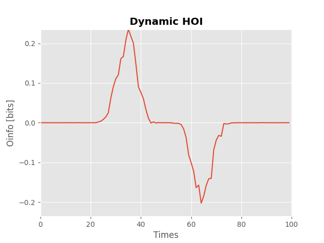
In the same way, we can simulate dynamic redundancy and synergy (i.e. the relationship between variables evolves over time). Here, we are going to use the same trick as above to simulate redundancy and synergy except that the relationship is going to be modulated by a temporal hanning window.

# simulate a dynamic network
x = np.random.rand(1000, 3, 100)

# define a window to modulate the interactions
win = np.hanning(30).reshape(1, -1)

# inject redundancy between samples [20, 50]
x_ref = x[:, 0, 20:50] * win
x[:, 1, 20:50] += x_ref
x[:, 2, 20:50] += x_ref

# inject synergy between samples [50, 80]
x[:, 0, 50:80] += win * (x[:, 1, 50:80] + x[:, 2, 50:80])

# compute the dynamic hoi
hoi = compute_hoi_beh(x)
h_max = max(abs(hoi.max()), abs(hoi.min()))

# plot the result
plt.plot(hoi)
plt.xlim(0.0, 100)
plt.ylim(-h_max, h_max)
plt.xlabel("Times")
plt.ylabel("Oinfo [bits]")
plt.title("Dynamic HOI", fontweight="bold")

  0%|          |  0/1 [00:00<?,       ?it/s]
100%|██████████| Oinfo (3):  1/1 [00:00<00:00,    2.35it/s]

Text(0.5, 1.0, 'Dynamic HOI')

Redundant and synergistic network encoding#

In this second part, we are going to switch for encoding measure, in the sens that elements of a network areg going to carry redundant or synergistic information about an external variable. To estimate HOI about a target variable Y, we’re going to use the hoi.metrics.GradientOinfo. To simulate redundancy and synergy, we’re going to use the same methods as before.

# function to estimate the nature of the interactions
def compute_hoi_enc(x, y):
    """This function computes the HOI using the Oinfo."""
    model = GradientOinfo(x, y)
    hoi = model.fit(method="gc", minsize=3, maxsize=3)
    return hoi.squeeze()

Simulating redundant encoding#

To simulate redundancy between a triplet of variable X and a target variable Y, we are going to use the same function as before hoi.simulation.simulate_hoi_gauss but this time, we are going to precise that we want a target by setting target=True.

# x = (n_samples, n_nodes)
x, y = simulate_hoi_gauss(
    target=True, n_samples=1000, triplet_character="redundancy"
)

compute hoi

hoi = compute_hoi_enc(x, y)

  0%|          |  0/1 [00:00<?,       ?it/s]
100%|██████████| Oinfo (3):  1/1 [00:00<00:00,    6.14it/s]


  0%|          |  0/1 [00:00<?,       ?it/s]
100%|██████████| Oinfo (3):  1/1 [00:00<00:00,    2.89it/s]

Print HOI value

print(f"HOI between nodes (1, 2, 3) about y : {hoi}")

HOI between nodes (1, 2, 3) about y : 0.17019176483154297

the estimated HOI is positive which represents redundant interactions between the three nodes about Y.

Simulating synergistic encoding#

Similarly, we can simulate a synergistic network encoding behavior by setting target=True and a synergistic behavior.

# x = (n_samples, n_nodes)
x, y = simulate_hoi_gauss(
    target=True, n_samples=1000, triplet_character="synergy"
)

compute hoi

hoi = compute_hoi_enc(x, y)

  0%|          |  0/1 [00:00<?,       ?it/s]
100%|██████████| Oinfo (3):  1/1 [00:00<00:00,    6.09it/s]


  0%|          |  0/1 [00:00<?,       ?it/s]
100%|██████████| Oinfo (3):  1/1 [00:00<00:00,    6.30it/s]

Print HOI value

print(f"HOI between nodes (1, 2, 3) about y : {hoi}")

HOI between nodes (1, 2, 3) about y : -1.9361505508422852

the estimated HOI is negative which represents synergistic interactions between the three nodes about Y.

Simulating redundant encoding by copy operation#

To simulate redundancy, we copy the Y variable into each node of X

# x = (n_samples, n_nodes)
x = np.random.rand(1000, 3)
y = np.random.rand(1000)

# inject y in all nodes
x[:, 0] += y
x[:, 1] += y
x[:, 2] += y

compute hoi

hoi = compute_hoi_enc(x, y)

  0%|          |  0/1 [00:00<?,       ?it/s]
100%|██████████| Oinfo (3):  1/1 [00:00<00:00,    6.11it/s]


  0%|          |  0/1 [00:00<?,       ?it/s]
100%|██████████| Oinfo (3):  1/1 [00:00<00:00,    6.25it/s]

Print HOI value

print(f"HOI between nodes (1, 2, 3) about y : {hoi}")

HOI between nodes (1, 2, 3) about y : 0.34401702880859375

the estimated HOI is positive which represents redundant interactions between the three nodes about Y.

Simulating synergistic encoding by sum operation#

To simulate synergy, we define the Y variable as the sum of the three nodes

# x = (n_samples, n_nodes)
x = np.random.rand(1000, 3)
y = x[:, 0] + x[:, 1] + x[:, 2]

compute hoi

hoi = compute_hoi_enc(x, y)

  0%|          |  0/1 [00:00<?,       ?it/s]
100%|██████████| Oinfo (3):  1/1 [00:00<00:00,    6.06it/s]


  0%|          |  0/1 [00:00<?,       ?it/s]
100%|██████████| Oinfo (3):  1/1 [00:00<00:00,    6.27it/s]

Print HOI value

print(f"HOI between nodes (1, 2, 3) about y : {hoi}")

HOI between nodes (1, 2, 3) about y : -2.223212242126465

the estimated HOI is negative which represents synergistic interactions between the three nodes about Y.

Simulating dynamic redundant and synergistic encoding#

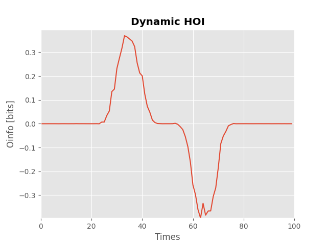
Finally, in the previous example, we used a static X and X. We can define a dynamic network and a dynamic target to simulate time-varying redundant and synergistic interactions about Y.

# simulate a dynamic network
x = np.random.rand(1000, 3, 100)
y = np.random.rand(1000, 1, 100)

# define a window to modulate the interactions
win = np.hanning(30).reshape(1, -1)

# inject redundancy between samples [20, 50]
x[:, [0], 20:50] += y[:, :, 20:50] * win
x[:, [1], 20:50] += y[:, :, 20:50] * win
x[:, [2], 20:50] += y[:, :, 20:50] * win


# inject synergy between samples [50, 80]
y[:, :, 50:80] += win * (
    x[:, [0], 50:80] + x[:, [1], 50:80] + x[:, [2], 50:80]
)

# compute the dynamic hoi
hoi = compute_hoi_enc(x, y)
h_max = max(abs(hoi.max()), abs(hoi.min()))

# plot the result
plt.plot(hoi)
plt.xlim(0.0, 100)
plt.ylim(-h_max, h_max)
plt.xlabel("Times")
plt.ylabel("Oinfo [bits]")
plt.title("Dynamic HOI", fontweight="bold")
plt.show()

  0%|          |  0/1 [00:00<?,       ?it/s]
100%|██████████| Oinfo (3):  1/1 [00:00<00:00,    4.54it/s]


  0%|          |  0/1 [00:00<?,       ?it/s]
100%|██████████| Oinfo (3):  1/1 [00:00<00:00,    3.61it/s]

Total running time of the script: (0 minutes 4.841 seconds)

Gallery generated by Sphinx-Gallery

How to simulate redundancy and synergy

Contents

How to simulate redundancy and synergy#

Redundant and synergistic network behavior#

Simulating synergistic behavior#

Simulating redundant behavior#

Simulating synergistic behavior by sum operation#

Simulating redundant behavior by copy operator#

Simulating dynamic redundancy and synergy#

Redundant and synergistic network encoding#

Simulating redundant encoding#

Simulating synergistic encoding#

Simulating redundant encoding by copy operation#

Simulating synergistic encoding by sum operation#

Simulating dynamic redundant and synergistic encoding#