Comparison of entropy estimators for various distributions

In this example, we are going to compare entropy estimators. In particular, some distributions, such as normal, uniform or exponential distributions lead to specific values of entropies. In this this tutorial we are going to :

1. Simulate data following either a normal, uniform or exponential distributions

2. Define several estimators of entropy

3. Compute the entropy for a varying number of samples

4. See if the computed entropies converge toward the theoretical value

import numpy as np

from hoi.core import get_entropy

import matplotlib.pyplot as plt

plt.style.use("ggplot")

Definition of estimators of entropy

Let us define several estimators of entropy. We are going to use the GC (Gaussian Copula), the KNN (k Nearest Neighbor), the kernel-based estimator and the histogram estimator.

# list of estimators to compare
metrics = {
    "GC": get_entropy("gc"),
    "Gaussian": get_entropy(method="gauss"),
    "Histogram": get_entropy(method="histogram"),
    "KNN-3": get_entropy("knn", k=3),
    "Kernel": get_entropy("kernel"),
}

# number of samples to simulate data
n_samples = np.geomspace(20, 1000, 15).astype(int)

# number of repetitions to estimate the percentile interval
n_repeat = 10


# plotting function
def plot(h_x, h_theoric):
    """Plotting function."""
    for n_m, metric_name in enumerate(h_x.keys()):
        # get the entropies
        x = h_x[metric_name]

        # get the color
        color = f"C{n_m}"

        # estimate lower and upper bounds of the [5, 95]th percentile interval
        x_low, x_high = np.percentile(x, [5, 95], axis=0)

        # plot the entropy as a function of the number of samples and interval
        plt.plot(n_samples, x.mean(0), color=color, lw=2, label=metric_name)
        plt.fill_between(n_samples, x_low, x_high, color=color, alpha=0.2)

    # plot the theoretical value
    plt.axhline(
        h_theoric, linestyle="--", color="k", label="Theoretical entropy"
    )
    plt.legend()
    plt.xlabel("Number of samples")
    plt.ylabel("Entropy [bits]")

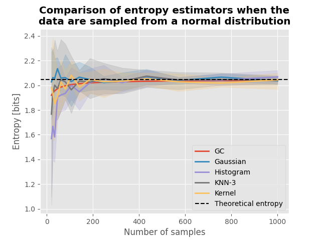
Entropy of data sampled from normal distribution

For data sampled from a normal distribution of mean m and standard deviation of σ (\(X \sim \mathcal{N}(0, 1)\)), the theoretical entropy is defined by :

\[H(X) = \frac{1}{2} \times log_{2}(2πeσ^2)\]

with e the Euler constant.

# mean and standard error N(0, 1)
mu = 0.0
sigma = 1.0

# define the theoretic entropy
h_theoric = 0.5 * np.log2(2 * np.pi * np.e * (sigma**2))

# compute entropies using various metrics
h_x = {k: np.zeros((n_repeat, len(n_samples))) for k in metrics.keys()}

for metric, fcn in metrics.items():
    for n_s, s in enumerate(n_samples):
        for n_r in range(n_repeat):
            x = np.random.normal(mu, sigma, size=(s,)).reshape(1, -1)
            h_x[metric][n_r, n_s] = fcn(x)

# plot the results
plot(h_x, h_theoric)
plt.title(
    "Comparison of entropy estimators when the\ndata are sampled from a "
    "normal distribution",
    fontweight="bold",
)
plt.show()

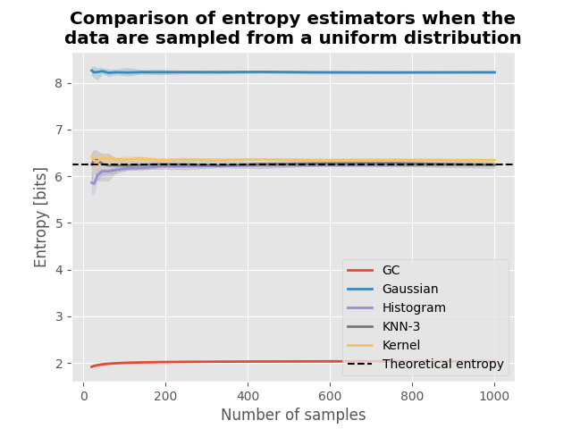
Entropy of data sampled from a uniform distribution

For data sampled from a uniform distribution defined between bounds \([a, b]\) (\(X \sim \mathcal{U}(a, b)\)), the theoretical entropy is defined by :

\[H(X) = log_{2}(b - a)\]

# boundaries
a = 31
b = 107

# define the theoretic entropy
h_theoric = np.log2(b - a)

# compute entropies using various metrics
h_x = {k: np.zeros((n_repeat, len(n_samples))) for k in metrics.keys()}

for metric, fcn in metrics.items():
    for n_s, s in enumerate(n_samples):
        for n_r in range(n_repeat):
            x = np.random.uniform(a, b, size=(s,)).reshape(1, -1)
            h_x[metric][n_r, n_s] = fcn(x)

# plot the results
plot(h_x, h_theoric)
plt.title(
    "Comparison of entropy estimators when the\ndata are sampled from a "
    "uniform distribution",
    fontweight="bold",
)
plt.show()

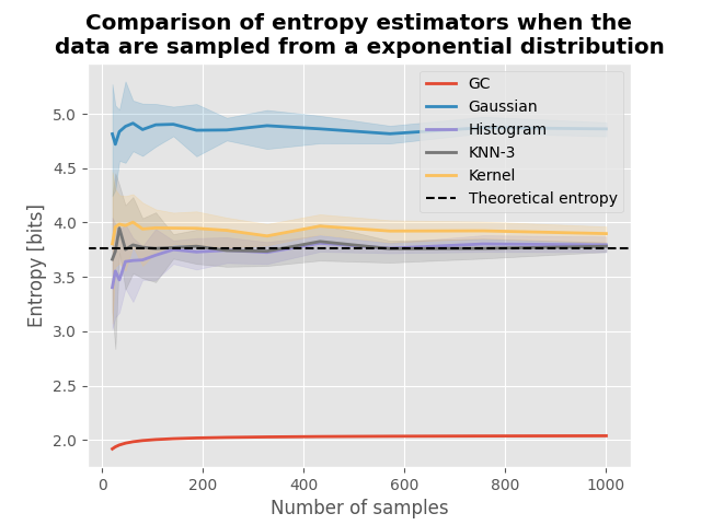
Entropy of data sampled from an exponential distribution

For data sampled from an exponential distribution defined by its rate \(lambda\), the theoretical entropy is defined by :

\[H(X) = log(e / \lambda)\]

# lambda parameter
lambda_ = 0.2

# define the theoretic entropy
h_theoric = np.log2(np.e / lambda_)

# compute entropies using various metrics
h_x = {k: np.zeros((n_repeat, len(n_samples))) for k in metrics.keys()}

for metric, fcn in metrics.items():
    for n_s, s in enumerate(n_samples):
        for n_r in range(n_repeat):
            x = np.random.uniform(a, b, size=(s,)).reshape(1, -1)
            x = np.random.exponential(1 / lambda_, size=(1, s)).reshape(1, -1)
            h_x[metric][n_r, n_s] = fcn(x)

# plot the results
plot(h_x, h_theoric)
plt.title(
    "Comparison of entropy estimators when the\ndata are sampled from a "
    "exponential distribution",
    fontweight="bold",
)
plt.show()