Topological Information : conditioning on orders

The following example highlights a metric known as “Topological Information” which was introduced by Baudot et al., 2019 [4]. This metric, founded on disparities in entropies, enables estimation of Higher Order Interactions while possessing the notable characteristic of being able to segregate specific orders. Specifically, when simulating redundancies at the third order utilizing the O-information metric (hoi.metrics.Oinfo), any quadruplets containing the superfluous triplet will yield redundancy. Conversely, the InfoTopo metric (hoi.metrics.InfoTopo) has the capability of pinpointing exclusively the redundant triplet. You can also check the original implementation of this estimator : https://infotopo.readthedocs.io/

import numpy as np

from hoi.metrics import InfoTopo, Oinfo
from hoi.utils import get_nbest_mult
from hoi.plot import plot_landscape

import matplotlib.pyplot as plt

plt.style.use("ggplot")

Simulate redundant and synergistic interactions

Let’s start by simulating a small network of 7 nodes with 1000 samples each. Then we’re going to introduce redundancy between the triplet (0, 1, 2) and synergy between the quadruplet (3, 4, 5, 6). For further information about how to simulate redundant and synergistic interactions, checkout the example How to simulate redundancy and synergy

# 7 nodes network with 1000 samples each
x = np.random.rand(1000, 7)

# redundant interactions between triplet of nodes (0, 1, 2)
x[:, 1] += x[:, 0]
x[:, 2] += x[:, 0]

# synergistic interactions between quadruplet of nodes (3, 4, 5, 6)
x[:, 3] += x[:, 4] + x[:, 5] + x[:, 6]

Spatial spreading : the problem with the O-information

Let’s compute the HOI using the O-information

model = Oinfo(x)
hoi = model.fit(minsize=3, method="gc")

  0%|          |  0/5 [00:00<?,       ?it/s]
 20%|██        | Oinfo (3):  1/5 [00:00<00:01,    2.72it/s]
 40%|████      | Oinfo (4):  2/5 [00:00<00:00,    3.22it/s]
 60%|██████    | Oinfo (5):  3/5 [00:01<00:00,    2.62it/s]
 80%|████████  | Oinfo (6):  4/5 [00:01<00:00,    2.42it/s]
100%|██████████| Oinfo (7):  5/5 [00:02<00:00,    2.45it/s]

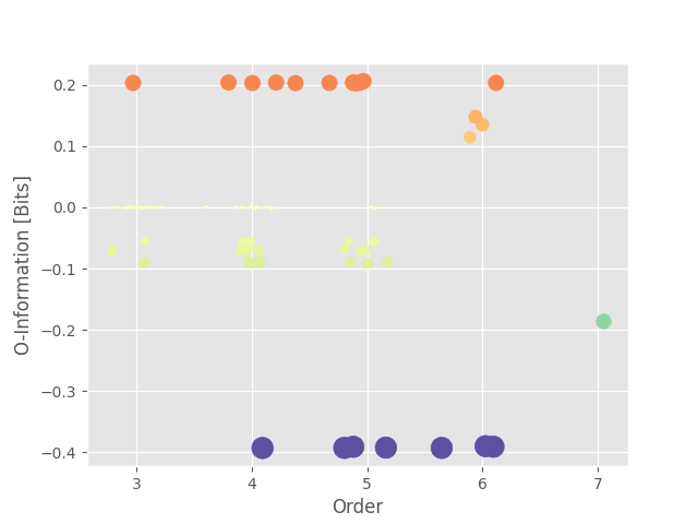
Now we can plot the landscape. This landscape show the values of HOI for different orders. As a reminder, for the O-information, positive values stand for redundant interactions while negative values stand for synergistic interactions.

plot_landscape(
    hoi,
    model=model,
    kind="scatter",
    plt_kwargs=dict(cmap="Spectral_r"),
    undersampling=False,
)
plt.show()

we can also print the multiplets with the highest values of O-information

print(get_nbest_mult(hoi, model=model))

   index  order       hoi           multiplet
0     70      5  0.205925     [0, 1, 2, 3, 4]
1     36      4  0.203808        [0, 1, 2, 4]
2     35      4  0.203772        [0, 1, 2, 3]
3     73      5  0.203644     [0, 1, 2, 4, 5]
4     72      5  0.203503     [0, 1, 2, 3, 6]
5     90      5 -0.390869     [2, 3, 4, 5, 6]
6     84      5 -0.392231     [0, 3, 4, 5, 6]
7     89      5 -0.392670     [1, 3, 4, 5, 6]
8     95      6 -0.392677  [0, 1, 3, 4, 5, 6]
9     69      4 -0.392874        [3, 4, 5, 6]

As we can see from the landscape and the printed table, the triplet (0, 1, 2) with redundant interactions is present in all of the multiplets of higher orders (order 4, 5, 6). Same thing holds with the synergistic quadruplets (3, 4, 5, 6). In short, the O-information can’t isolate both multiplets.

Multiplet isolation using the Topological Information

In contrast to the O-information, the Topological Information is based on conditional mutual information and conditioned on lower orders. This conditioning should, in theory, avoid the spatial spreading. The mathematical definition of the Topological Information is given by :

\[I_{k}(X_{1}; ...; X_{k}) = \sum_{i=1}^{k} (-1)^{i - 1} \sum_{ I\subset[k];card(I)=i} H_{i}(X_{I})\]

model = InfoTopo(x)
hoi = model.fit(minsize=3, method="gc")

  0%|          |  0/7 [00:00<?,       ?it/s]
 14%|█▍        | Entropy H(1):  1/7 [00:00<00:00,    7.78it/s]
 29%|██▊       | Entropy H(2):  2/7 [00:00<00:00,    7.62it/s]
 43%|████▎     | Entropy H(3):  3/7 [00:00<00:00,    7.65it/s]
 57%|█████▋    | Entropy H(4):  4/7 [00:00<00:00,    8.07it/s]
 71%|███████▏  | Entropy H(5):  5/7 [00:00<00:00,    8.38it/s]
 86%|████████▌ | Entropy H(6):  6/7 [00:00<00:00,    8.59it/s]
100%|██████████| Entropy H(7):  7/7 [00:00<00:00,    8.77it/s]


Mutual information:   0%|          | 0/99 [00:00<?, ?it/s]


Mutual information: 100%|██████████| 99/99 [00:00<00:00, 27892.53it/s]

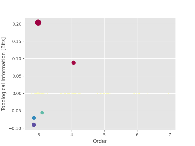
Again, we can plot the landscape. This time, as we can see, there’s no more spatial spreading. There are only two points and, using the printed table below, we can see that those two points correspond to our two multiplets (0, 1, 2) and (3, 4, 5, 6). However, the Topological Information did not correctly inferred the type of interactions as the quadruplet (3, 4, 5, 6) is identified as a redundant multiplet despite being synergistic.

plot_landscape(
    hoi,
    model=model,
    kind="scatter",
    plt_kwargs=dict(cmap="Spectral_r"),
    undersampling=False,
)
plt.show()

print(get_nbest_mult(hoi, model=model))

   index  order       hoi     multiplet
0      0      3  0.203173     [0, 1, 2]
1     69      4  0.087830  [3, 4, 5, 6]
2     25      3  0.001332     [2, 3, 4]
3      6      3  0.000945     [0, 2, 4]
4     26      3  0.000795     [2, 3, 5]
5     36      4 -0.000955  [0, 1, 2, 4]
6      2      3 -0.001291     [0, 1, 4]
7     33      3 -0.055869     [3, 5, 6]
8     31      3 -0.070711     [3, 4, 5]
9     32      3 -0.090620     [3, 4, 6]