Integrated Information Decomposition

This example illustrates how to use and interpret synergy and redundancy as defined in the Integrated Information Decomposition framework

import matplotlib.pyplot as plt
import numpy as np

from hoi.metrics import RedundancyphiID, AtomsPhiID
from hoi.utils import get_nbest_mult

plt.style.use("ggplot")

Definition

The Integrated Information decomposition framework (phiID) was introduced by Mediano et al (2021) [] to obtain a detailed description of information dynamics. One of the atoms of this decomposition, that received particular attention in the literature, are the synergy -> synergy atom (sts) and the redundancy -> redundancy atom (rtr). To compute these two atoms, one needs first to estimate the rtr atom, which can be done using the Minumum Mutual Information (MMI) approach, as:

\[Red(X,Y) = min (I(X_{t-\tau}; Y_{t}), I(X_{t-\tau}; X_t), I(Y_{t-\tau}; X_t), I(Y_{t-\tau}; Y_t))\]

rtr relates to the amount of information the two variables share about their own future. sts instead relate to the amount of information the two variables provide about their joint future.

Simulate synergy

A very simple way to simulate synergy is by to start with two independent variables and inflate autocorrelation by variables \(X_{1}, X_{2}, X_{3}\) receive a copy of a variable \(Y\), we will observe redundancy between \(X_{1}, X_{2}, X_{3}\) and \(Y\).

# lets start by simulating a variable x with 200 samples and 7 features
x = np.random.rand(200, 7)

# now to create synergy between the two first features, we do the following:
# to create interdependencies between past and future we use a uniform
# kernel in the following way

for i in range(190):
    x[i, 0] = np.sum(x[i : i + 20, 1]) + 0.2 * np.sum(x[i : i + 20, 0])
    x[i, 1] = np.sum(x[i : i + 20, 0]) + 0.2 * np.sum(x[i : i + 20, 1])

# define the sts model and launch it (AtomsPhiID return by default sts)
model = AtomsPhiID(x)
hoi = model.fit(minsize=2, maxsize=2)

# now we can take a look at the multiplets with the highest and lowest values
# of synergy. We will only select the multiplets of size 2 here
df = get_nbest_mult(hoi, model=model, minsize=2, maxsize=2, n_best=3)
print(df)

  0%|          |  0/1 [00:00<?,       ?it/s]
100%|██████████| SynPhiIDMMI order 2:  1/1 [00:00<00:00,    1.27it/s]

   index  order       hoi multiplet
0      0      2  0.845804    [0, 1]
1     11      2  0.010318    [2, 3]
2     19      2  0.006428    [4, 6]

as you see from the printed table, the couple of variables with the highest synergy is [0,1]

Simulate redundancy

# simulate x again
x = np.random.rand(200, 7)

# now to create redundancy between the two first features, we do the following:
# to create interdependencies between past and future we use a uniform
# kernel in the following way

for i in range(190):
    x[i, 0] = np.sum(x[i : i + 20, 1])

# Redundancy emerges when the two variables carry the same information about
# Their future. This can be achieved by copy operation between the two
# variables plus some noise.

x[:, 1] = x[:, 0] + np.random.rand(200) * 0.05

# define the redundancyphiID, launch it and inspect the best multiplets
model = RedundancyphiID(x)
hoi = model.fit(minsize=2, maxsize=2)
df = get_nbest_mult(hoi, model=model, minsize=2, maxsize=2, n_best=3)
print(df)

  0%|          |  0/1 [00:00<?,       ?it/s]
100%|██████████| RedPhiIDMMI order 2:  1/1 [00:00<00:00,    5.82it/s]

   index  order       hoi multiplet
0      0      2  1.698441    [0, 1]
1      1      2  0.002837    [0, 2]
2      6      2  0.002837    [1, 2]

This time, as expected, the two most redundant couple of variable is [0,1]

Combining redundancy and synergy

# simulate the variable x
n_features = 7
x = np.random.rand(200, n_features)

# synergy between (0, 1)
for i in range(190):
    x[i, 0] = np.sum(x[i : i + 20, 1]) + 0.1 * np.sum(x[i : i + 20, 0])
    x[i, 1] = np.sum(x[i : i + 20, 0]) + 0.1 * np.sum(x[i : i + 20, 1])

# redundancy between (0, 2), this will inject also synergy between
# variables 1 and 2

x[:, 2] = x[:, 0] + np.random.rand(200) * 0.05

define the AtomsPhiID, launch it and inspect the best couples of variables

model = AtomsPhiID(x)
syn_results = model.fit(minsize=2, maxsize=2)
df = get_nbest_mult(hoi, model=model, minsize=2, maxsize=2, n_best=3)
print(df)

# store the results in a matrix

matrix_to_plot = np.zeros((n_features, n_features))
for i, tup in enumerate(model.get_combinations(minsize=2, maxsize=2)[0]):
    m, g = tup
    matrix_to_plot[m, g] = syn_results[i][0]

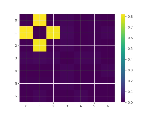
# plot the results matrix simmetrized

plt.imshow(
    matrix_to_plot + matrix_to_plot.T, aspect="auto", interpolation="none"
)
plt.colorbar()
plt.show()

  0%|          |  0/1 [00:00<?,       ?it/s]
100%|██████████| SynPhiIDMMI order 2:  1/1 [00:00<00:00,    1.83it/s]

   index  order       hoi multiplet
0      0      2  1.698441    [0, 1]
1      1      2  0.002837    [0, 2]
2      6      2  0.002837    [1, 2]

define the RedundancyphiID, launch it and inspect the best couples of variables (smilar results can be obtained using AtomsPhiID, with atom=’rtr’)

model = RedundancyphiID(x)
red_results = model.fit(minsize=2, maxsize=2)
df = get_nbest_mult(red_results, model=model, minsize=2, maxsize=2, n_best=3)
print(df)

# store the results in a matrix

matrix_to_plot = np.zeros((n_features, n_features))
for i, tup in enumerate(model.get_combinations(minsize=2, maxsize=2)[0]):
    m, g = tup
    matrix_to_plot[m, g] = red_results[i][0]

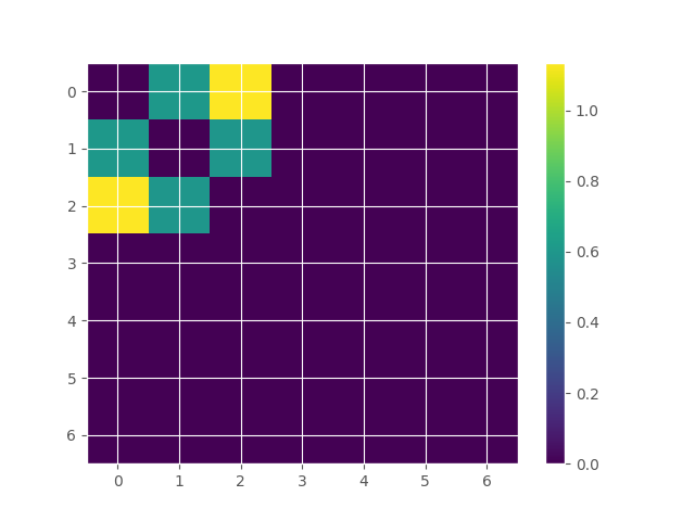
# plot the results matrix

plt.imshow(
    matrix_to_plot + matrix_to_plot.T, aspect="auto", interpolation="none"
)
plt.colorbar()
plt.show()

  0%|          |  0/1 [00:00<?,       ?it/s]
100%|██████████| RedPhiIDMMI order 2:  1/1 [00:00<00:00,    5.78it/s]

   index  order       hoi multiplet
0      1      2  1.134994    [0, 2]
1      0      2  0.603431    [0, 1]
2      6      2  0.597383    [1, 2]