Redundancy and Synergy MMI

This example illustrates how to use and interpret synergy and redundancy computed using the Minimum Mutual Information (MMI) approach to approximate the redundancy.

import numpy as np

from hoi.metrics import SynergyMMI, RedundancyMMI
from hoi.utils import get_nbest_mult
from hoi.plot import plot_landscape

import matplotlib.pyplot as plt

plt.style.use("ggplot")

Definition

Synergy and redundancy measures directly, respectively the ammount of synergy and redundancy carried by a group of variable \(S\) about a target variable \(Y\). Synergy is defined as follow :

\[Syn(S; Y) \equiv I(S; Y) - \max_{x_{i}\in S} I(S_{-i}; Y)\]

with : \(S = x_{1}, ..., x_{n}\) and \(S_{-i} = x_{1}, ..., x_{i-1}, x_{1+1}, ..., x_{n}\)

Positive values of Synergy stand for the presence of an higher information about \(Y\) when considering all the variables in \(S\) with respect to when considering only a subgroup of \(n-1\).

Redundancy, in the approximation based on the Minimum Mutual Information (MMI) framework, is computed as follow :

\[Red(S; Y) \equiv \min_{x_{i}\in S} I(X_{i}; Y)\]

Simulate univariate redundancy

A very simple way to simulate redundancy is to observe that if a triplet of variables \(X_{1}, X_{2}, X_{3}\) receive a copy of a variable \(Y\), we will observe redundancy between \(X_{1}, X_{2}, X_{3}\) and \(Y\). For further information about how to simulate redundant and synergistic interactions, checkout the example How to simulate redundancy and synergy.

# lets start by simulating a variable x with 200 samples and 7 features
x = np.random.rand(200, 7)

# now we can also generate a univariate random variable `Y`
y = np.random.rand(x.shape[0])

# we now send the variable y in the column (1, 3, 5) of `X`
x[:, 1] += y
x[:, 3] += y
x[:, 5] += y

# define the RSI model and launch it
model = RedundancyMMI(x, y)
hoi = model.fit(minsize=3, maxsize=5)

# now we can take a look at the multiplets with the highest and lowest values
# of RSI. We will only select the multiplets of size 3 here
df = get_nbest_mult(hoi, model=model, minsize=3, maxsize=3, n_best=3)
print(df)

  0%|          |  0/3 [00:00<?,       ?it/s]
 33%|███▎      | RedMMI order 3:  1/3 [00:00<00:00,    7.34it/s]
100%|██████████| RedMMI order 5:  3/3 [00:00<00:00,   18.31it/s]

   index  order       hoi  multiplet
0     20      3  0.392336  [1, 3, 5]
1     15      3  0.009812  [1, 2, 3]
2     26      3  0.009812  [2, 3, 5]

as you see from the printed table, the multiplet with the lowest (i.e. the most redundant multiplets) is (1, 3, 5).

Simulate multivariate redundancy

In the example above, we simulated a univariate \(Y\) variable (i.e. single column). However, it’s possible to simulate a multivariate variable.

# simulate x again
x = np.random.rand(200, 7)

# simulate a bivariate y variable
y = np.c_[np.random.rand(x.shape[0]), np.random.rand(x.shape[0])]

# we introduce redundancy between the triplet (1, 3, 5) and the first column of
# `Y` and between (0, 2, 6) and the second column of `Y`.
x[:, 1] += y[:, 0]
x[:, 3] += y[:, 0]
x[:, 5] += y[:, 0]
x[:, 0] += y[:, 1]
x[:, 2] += y[:, 1]
x[:, 6] += y[:, 1]

# define the Redundancy, launch it and inspect the best multiplets
model = RedundancyMMI(x, y)
hoi = model.fit(minsize=3, maxsize=5)
df = get_nbest_mult(hoi, model=model, minsize=3, maxsize=3, n_best=5)
print(df)

  0%|          |  0/3 [00:00<?,       ?it/s]
 33%|███▎      | RedMMI order 3:  1/3 [00:00<00:00,    7.07it/s]

   index  order       hoi  multiplet
0     27      3  0.483097  [2, 3, 6]
1     33      3  0.444745  [3, 5, 6]
2     26      3  0.444745  [2, 3, 5]
3     30      3  0.444745  [2, 5, 6]
4     14      3  0.420686  [0, 5, 6]

It is important to notice that in this case the redundancy it is not able to find only the two multiplets in which we generate redundancy, but instead all the possible combination of the six variables in which a part of Y was copied are resulting redundant. This follows directly by the definition of redundancy with the MMI approximation. It is important to remember this limitation when leveraging its results and eventually consider a double check with other metrics, as RSI or O-information gradient.

Simulate univariate and multivariate synergy

Lets move on to the simulation of synergy that is a bit more subtle. One way of simulating synergy is to go the other way of redundancy, meaning we are going to add features of x inside Y. That way, we can only retrieve the Y variable by knowing the subset of X.

# simulate the variable x
x = np.random.rand(200, 7)

# synergy between (0, 3, 5) and 5
y = x[:, 0] + x[:, 3] + x[:, 5]

# define the Synergy, launch it and inspect the best multiplets
model = SynergyMMI(x, y)
hoi = model.fit(minsize=3, maxsize=5)
df = get_nbest_mult(hoi, model=model, minsize=3, maxsize=3, n_best=3)
print(df)

  0%|          |  0/3 [00:00<?,       ?it/s]
 33%|███▎      | SynMMI order 3:  1/3 [00:00<00:00,    3.63it/s]
 67%|██████▋   | SynMMI order 4:  2/3 [00:00<00:00,    3.62it/s]
100%|██████████| SynMMI order 5:  3/3 [00:00<00:00,    3.64it/s]

   index  order           hoi  multiplet
0     10      3  1.365911e+00  [0, 3, 5]
1     33      3  1.236016e-02  [3, 5, 6]
2     12      3  5.705744e-03  [0, 4, 5]
3     27      3 -3.439481e-08  [2, 3, 6]

as we can see here, the highest values of higher-order interactions (i.e. synergy) is achieved for the multiplet (0, 3, 5). Now we can do the same for multivariate synergy.

# simulate the variable `X`
x = np.random.rand(200, 7)

# simulate y and introduce synergy between the subset (0, 3, 5) of `X` and the
# subset (1, 2, 6)
y = np.c_[x[:, 0] + x[:, 3] + x[:, 5], x[:, 1] + x[:, 2] + x[:, 6]]

# define the Synergy, launch it and inspect the best multiplets
model = SynergyMMI(x, y)
hoi = model.fit(minsize=3, maxsize=5)
df = get_nbest_mult(hoi, model=model, minsize=3, maxsize=3, n_best=3)
print(df)

  0%|          |  0/3 [00:00<?,       ?it/s]
 33%|███▎      | SynMMI order 3:  1/3 [00:00<00:00,    3.52it/s]
 67%|██████▋   | SynMMI order 4:  2/3 [00:00<00:00,    3.39it/s]
100%|██████████| SynMMI order 5:  3/3 [00:00<00:00,    3.39it/s]

   index  order       hoi  multiplet
0     18      3  1.600548  [1, 2, 6]
1     10      3  1.533365  [0, 3, 5]
2     21      3  0.329931  [1, 3, 6]

Combining redundancy and synergy

# simulate the variable x and y
x = np.random.rand(200, 7)
y = np.random.rand(200, 2)

# synergy between (0, 1, 2) and the first column of `Y`
y[:, 0] = x[:, 0] + x[:, 1] + x[:, 2]

# redundancy between (3, 4, 5) and the second column of `X`
x[:, 3] = y[:, 1]
x[:, 4] = y[:, 1]
x[:, 5] = y[:, 1]

# define the Synergy, launch it and inspect the best multiplets
model_syn = SynergyMMI(x, y)
hoi_syn = model_syn.fit(minsize=3, maxsize=5)
df = get_nbest_mult(hoi_syn, model=model, minsize=3, maxsize=3, n_best=3)
print(" ")
print("Synergy results")
print(" ")
print(df)

# define the Synergy, launch it and inspect the best multiplets
model_red = RedundancyMMI(x, y)
hoi_red = model_red.fit(minsize=3, maxsize=5)
df = get_nbest_mult(hoi_red, model=model, minsize=3, maxsize=3, n_best=3)
print(" ")
print("Redundancy results")
print(" ")
print(df)

  0%|          |  0/3 [00:00<?,       ?it/s]
 33%|███▎      | SynMMI order 3:  1/3 [00:00<00:00,    3.61it/s]
 67%|██████▋   | SynMMI order 4:  2/3 [00:00<00:00,    3.54it/s]
100%|██████████| SynMMI order 5:  3/3 [00:00<00:00,    3.45it/s]


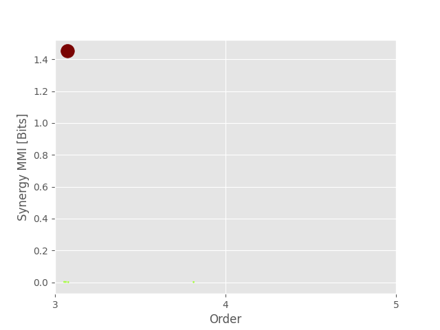
Synergy results

   index  order       hoi  multiplet
0      0      3  1.450861  [0, 1, 2]
1     18      3  0.002443  [1, 2, 6]
2      8      3  0.002230  [0, 2, 6]

  0%|          |  0/3 [00:00<?,       ?it/s]
 33%|███▎      | RedMMI order 3:  1/3 [00:00<00:00,    7.01it/s]


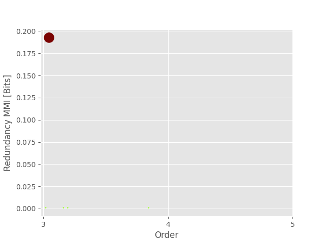
Redundancy results

   index  order       hoi  multiplet
0      0      3  0.192637  [0, 1, 2]
1      4      3  0.000867  [0, 1, 6]
2      8      3  0.000867  [0, 2, 6]

Plotting redundancy

plot_landscape(
    hoi_red,
    model_red,
    kind="scatter",
    undersampling=False,
    plt_kwargs=dict(cmap="turbo"),
)

plt.show()

Plotting synergy

plot_landscape(
    hoi_syn,
    model_syn,
    kind="scatter",
    undersampling=False,
    plt_kwargs=dict(cmap="turbo"),
)

plt.show()