Defining a custom estimator

This example illustrates how to define a custom estimator for measuring information. In particular, we are going to define estimators from the field of machine-learning by means of decoding and regression.

import numpy as np
import xarray as xr

from frites.estimator import CustomEstimator

from sklearn.discriminant_analysis import LinearDiscriminantAnalysis
from sklearn.linear_model import LinearRegression
from sklearn.model_selection import cross_val_score
from frites import set_mpl_style

import matplotlib.pyplot as plt
set_mpl_style()

Custom estimator : decoders

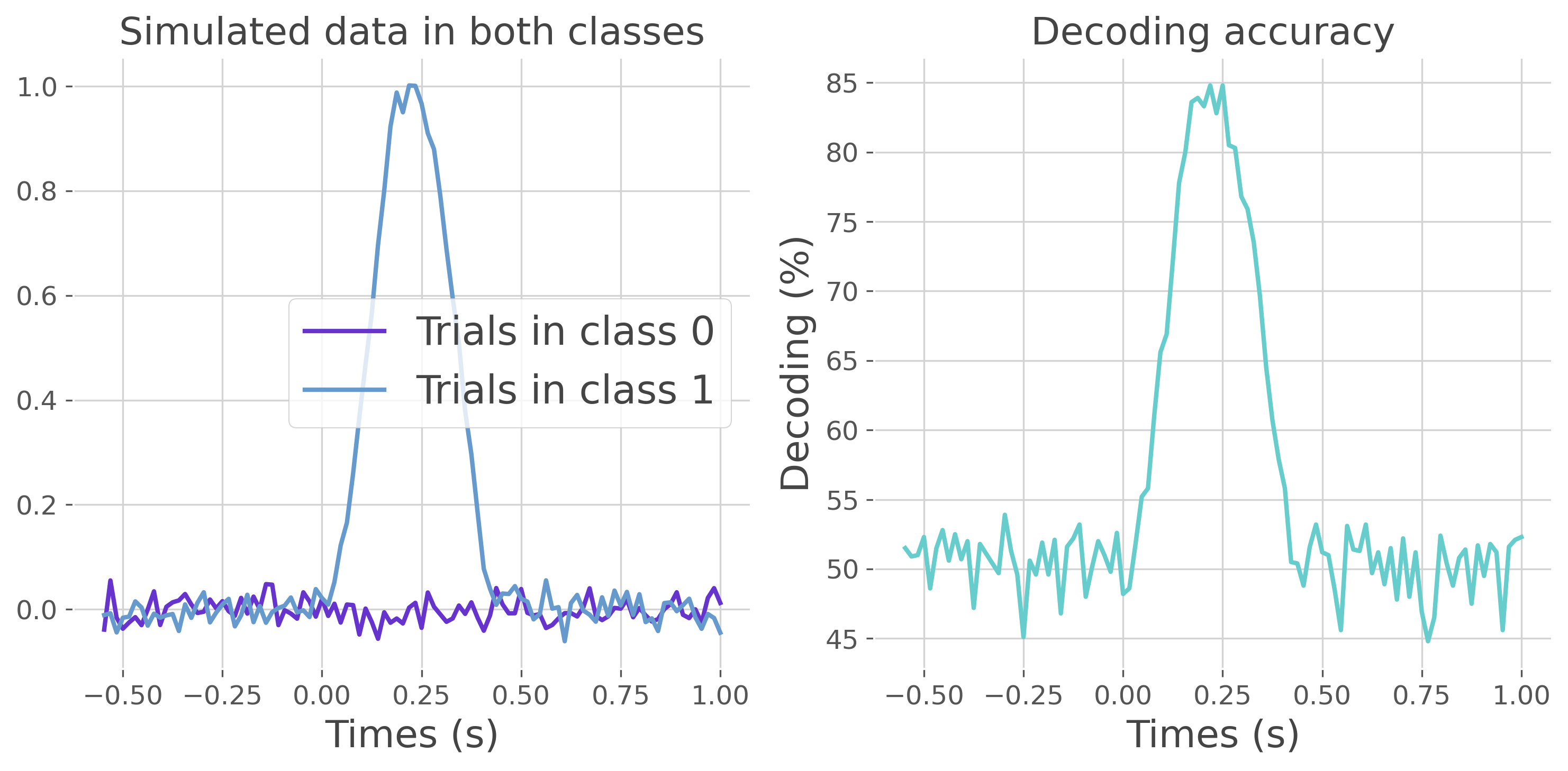
This first part introduces how to define custom estimators in order to classify conditions.

# main decoding function
def classify(x, y):
    """Classify conditions for 3D variables.

    x.shape = (n_var, 1, n_samples)
    y.shape = (n_var, 1, n_samples)
    """
    # define the decoder to use
    decoder = LinearDiscriminantAnalysis()

    # classify each point
    n_var = x.shape[0]
    decoding = np.zeros((n_var,))
    for n in range(n_var):
        d = cross_val_score(decoder, x[n, :, :].T, y[n, 0, :], cv=10, n_jobs=1)
        decoding[n] = d.mean() * 100.
    return decoding

# data simulation
n_trials = 1000
n_times = 100
times = (np.arange(n_times) - 35) / 64.
half_trials = int(np.round(n_trials / 2))

x = np.random.normal(scale=.5, size=(n_times, 1, n_trials))
x[35:65, :, half_trials::] += np.hanning(30).reshape(-1, 1, 1)
y = np.array([0] * half_trials + [1] * half_trials)


# define the custom estimator
name = 'Decoder estimator'
mi_type = 'cd'  # decoding a continuous variable based on a discrete one
multivariate = False  # estimator is designed for univariate inputs
est = CustomEstimator(name, mi_type, classify, multivariate=multivariate)

# run the estimator
decoding = est.estimate(x, y).squeeze()

# plot the result
plt.figure(figsize=(10, 5))

plt.subplot(1, 2, 1)
x = xr.DataArray(x, dims=('times', 'mv', 'trials'), coords=(times, [0], y))
x_gp = x.groupby('trials').mean('trials').squeeze()
plt.plot(times, x_gp.sel(trials=0), color='#6633cc', label='Trials in class 0',
         lw=2)
plt.plot(times, x_gp.sel(trials=1), color='#6699cc', label='Trials in class 1',
         lw=2)
plt.legend()
plt.xlabel('Times (s)')
plt.title("Simulated data in both classes")

plt.subplot(1, 2, 2)
plt.plot(times, decoding, lw=2, color='#66cccc')
plt.xlabel('Times (s)')
plt.ylabel('Decoding (%)')
plt.title('Decoding accuracy')
plt.tight_layout()

plt.show()

Custom estimator : regression

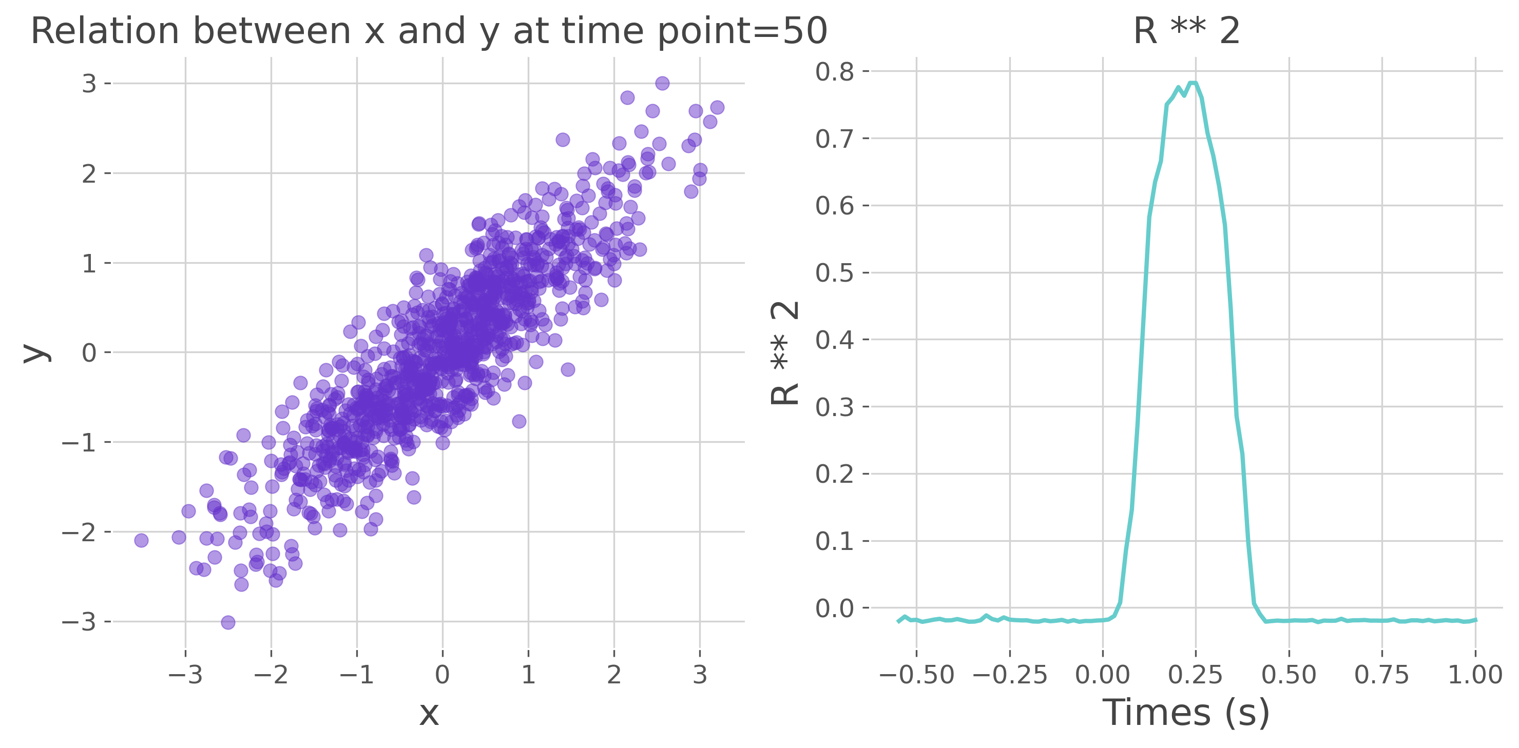
This second part introduces how to define custom estimators in order to perform regressions.

# main decoding function
def regression(x, y):
    """Regression between x and y variables.

    x.shape = (n_var, 1, n_samples)
    y.shape = (n_var, 1, n_samples)
    """
    # define the regression to use
    regressor = LinearRegression()

    # classify each point
    n_var = x.shape[0]
    regr = np.zeros((n_var,))
    for n in range(n_var):
        d = cross_val_score(regressor, x[n, :, :].T, y[n, 0, :], cv=10,
                            n_jobs=1, scoring='r2')
        regr[n] = d.mean()
    return regr


# data simulation
n_trials = 1000
n_times = 100
times = (np.arange(n_times) - 35) / 64.

x = np.random.normal(scale=.5, size=(n_times, 1, n_trials))
y = np.random.normal(size=(n_trials,))
x[35:65, ...] += y.reshape(1, 1, -1) * np.hanning(30).reshape(-1, 1, 1)

# define the custom estimator
name = 'Regression estimator'
mi_type = 'cc'  # regression between two continuous variables
multivariate = False  # estimator is designed for univariate inputs
est = CustomEstimator(name, mi_type, regression, multivariate=multivariate)

# run the estimator
regr = est.estimate(x, y).squeeze()

# plot the result
plt.figure(figsize=(10, 5))

plt.subplot(1, 2, 1)
plt.scatter(x[50, 0, :], y, alpha=.5, s=40, color='#6633cc')
plt.xlabel('x')
plt.ylabel('y')
plt.title("Relation between x and y at time point=50")

plt.subplot(1, 2, 2)
plt.plot(times, regr, lw=2, color='#66cccc')
plt.xlabel('Times (s)')
plt.ylabel('R ** 2')
plt.title('R ** 2')
plt.tight_layout()

plt.show()

Estimated memory usage: 31 MB