MI between two continuous variables

This example illustrates how to compute the mutual information between two continuous variables and also perform statistics. Usually, the first variable is an electrophysiological data (M/EEG, intracranial) and a regressor. This kind of mutual information is equivalent to a traditional correlation. Note that the regressor variable can either be univariate (single column) or multivariate (multiple columns). For further details, see Ince et al., 2017 [12]

import numpy as np

from frites.simulations import sim_multi_suj_ephy, sim_mi_cc
from frites.dataset import DatasetEphy
from frites.workflow import WfMi
from frites import set_mpl_style

import matplotlib.pyplot as plt
set_mpl_style()

Simulate electrophysiological data

Let’s start by simulating MEG / EEG electrophysiological data coming from multiple subjects using the function frites.simulations.sim_multi_suj_ephy(). As a result, the x output is a list of length n_subjects of arrays, each one with a shape of n_epochs, n_sites, n_times

modality = 'meeg'
n_subjects = 5
n_epochs = 400
n_times = 100
x, roi, time = sim_multi_suj_ephy(n_subjects=n_subjects, n_epochs=n_epochs,
                                  n_times=n_times, modality=modality,
                                  random_state=0)

Extract the regressor variable

Once we have the electrophysiological, we need to extract the second variable that is going to serves for computing the “correlation” at each time point and at each site / channel / sensor. To do this, we can simply take the mean over time points and region of interest in a time window

sl = slice(40, 60)
y = [x[k][..., sl].mean(axis=(1, 2)) for k in range(len(x))]

Note

Taking the mean across time points and space is exactly the behavior of the function frites.simulations.sim_mi_cc()

Define the electrophysiological dataset

Now we define an instance of frites.dataset.DatasetEphy

dt = DatasetEphy(x.copy(), y=y, roi=roi, times=time)

Compute the mutual information

Once we have the dataset instance, we can then define an instance of workflow frites.workflow.WfMi. This instance is used to compute the mutual information

# mutual information type ('cc' = continuous / continuous)
mi_type = 'cc'

# define the workflow
wf = WfMi(mi_type, inference='ffx')
# compute the mutual information without permutations
mi, _ = wf.fit(dt, mcp=None)

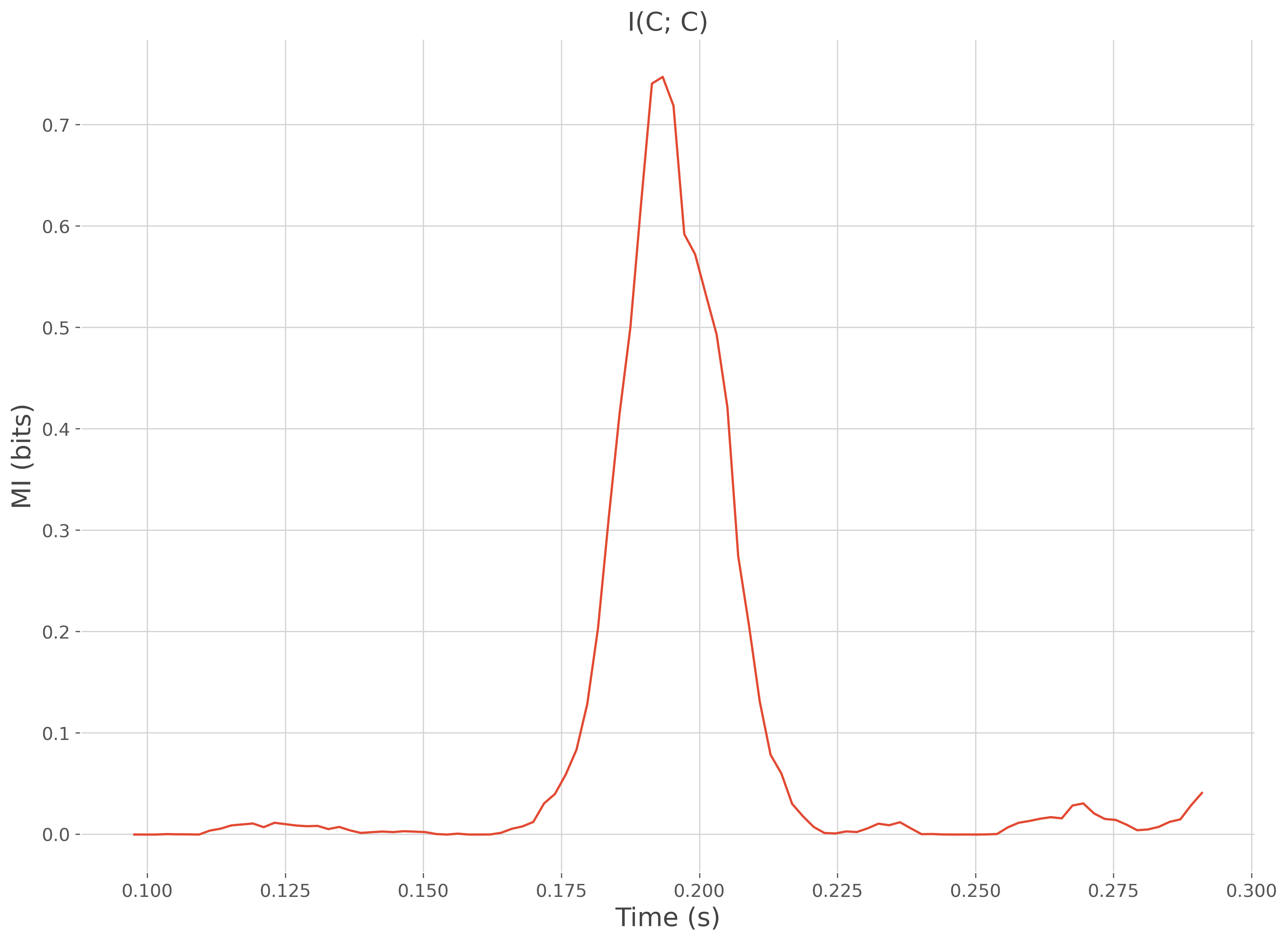
# plot the information shared between the data and the regressor y
plt.plot(time, mi)
plt.xlabel("Time (s)"), plt.ylabel("MI (bits)")
plt.title('I(C; C)')
plt.show()

  0%|          | Estimating MI : 0/1 [00:00<?,       ?it/s]
100%|██████████| Estimating MI : 1/1 [00:00<00:00,   12.21it/s]
100%|██████████| Estimating MI : 1/1 [00:00<00:00,   12.09it/s]

Evaluate the statistics

In the section above, the input parameter stat_method=None specifies that no statistics are going to be computed. Here, we show how to compute either within (ffx) or between subject (rfx) statistics.

mi_type = 'cc'
n_perm = 200
y, _ = sim_mi_cc(x, snr=.1)

# within subject statistics (ffx=fixed-effect)
ffx_stat = 'ffx_cluster_tfce'
dt_ffx = DatasetEphy(x.copy(), y=y, roi=roi, times=time)
wf_ffx = WfMi(mi_type=mi_type, inference='ffx')
mi_ffx, pv_ffx = wf_ffx.fit(dt_ffx, mcp='cluster', cluster_th='tfce',
                            n_perm=n_perm, n_jobs=1)

# between-subject statistics (rfx=random-effect)
dt_rfx = DatasetEphy(x.copy(), y=y, roi=roi, times=time)
wf_rfx = WfMi(mi_type=mi_type, inference='rfx')
mi_rfx, pv_rfx = wf_rfx.fit(dt_rfx, mcp='cluster', cluster_th='tfce',
                            n_perm=n_perm, n_jobs=1)

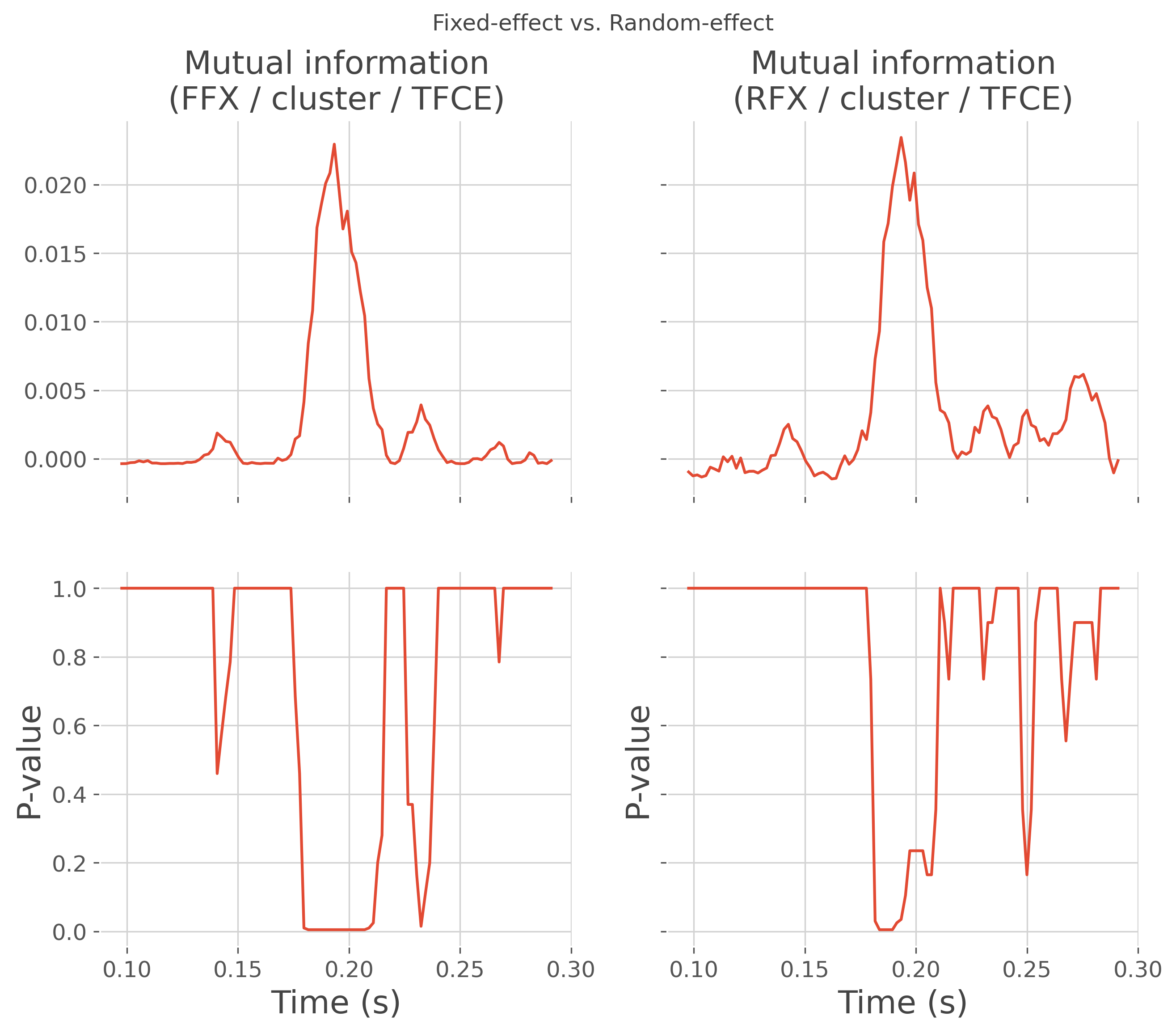
# plot the comparison
fig, axs = plt.subplots(nrows=2, ncols=2, sharex=True, sharey='row',
                        figsize=(10, 8))
fig.suptitle("Fixed-effect vs. Random-effect")

plt.sca(axs[0, 0])
plt.plot(time, mi_ffx)
plt.title(f"Mutual information\n(FFX / cluster / TFCE)")
plt.sca(axs[1, 0])
plt.plot(time, pv_ffx)
plt.xlabel("Time (s)"), plt.ylabel("P-value")
plt.sca(axs[0, 1])
plt.plot(time, mi_rfx)
plt.title(f"Mutual information\n(RFX / cluster / TFCE)")
plt.sca(axs[1, 1])
plt.plot(time, pv_rfx)
plt.xlabel("Time (s)"), plt.ylabel("P-value")
plt.show()

  0%|          | Estimating MI : 0/1 [00:00<?,       ?it/s]
100%|██████████| Estimating MI : 1/1 [00:00<00:00,    2.21it/s]
100%|██████████| Estimating MI : 1/1 [00:00<00:00,    2.21it/s]

  0%|          | Estimating MI : 0/1 [00:00<?,       ?it/s]
100%|██████████| Estimating MI : 1/1 [00:01<00:00,    1.77s/it]
100%|██████████| Estimating MI : 1/1 [00:01<00:00,    1.77s/it]

Estimated memory usage: 76 MB