FIT: Feature specific information transfer

This example illustrates how to compute Feature-specific Information Transfer (FIT), quantifying how much information about a specific feature flows between two regions. FIT merges the Wiener-Granger causality principle with information-content specificity. The theoretical background is described in [1] and the FIT is computed using the frites.conn.conn_fit() function. [1] Celotto M, et al. (2023) An information-theoretic quantification of the content of communication between brain regions. https://www.biorxiv.org/content/10.1101/2023.06.14.544903v1

import numpy as np
import xarray as xr

from frites.simulations import StimSpecAR
from frites.conn import conn_fit

from frites import set_mpl_style

import matplotlib.pyplot as plt
set_mpl_style()

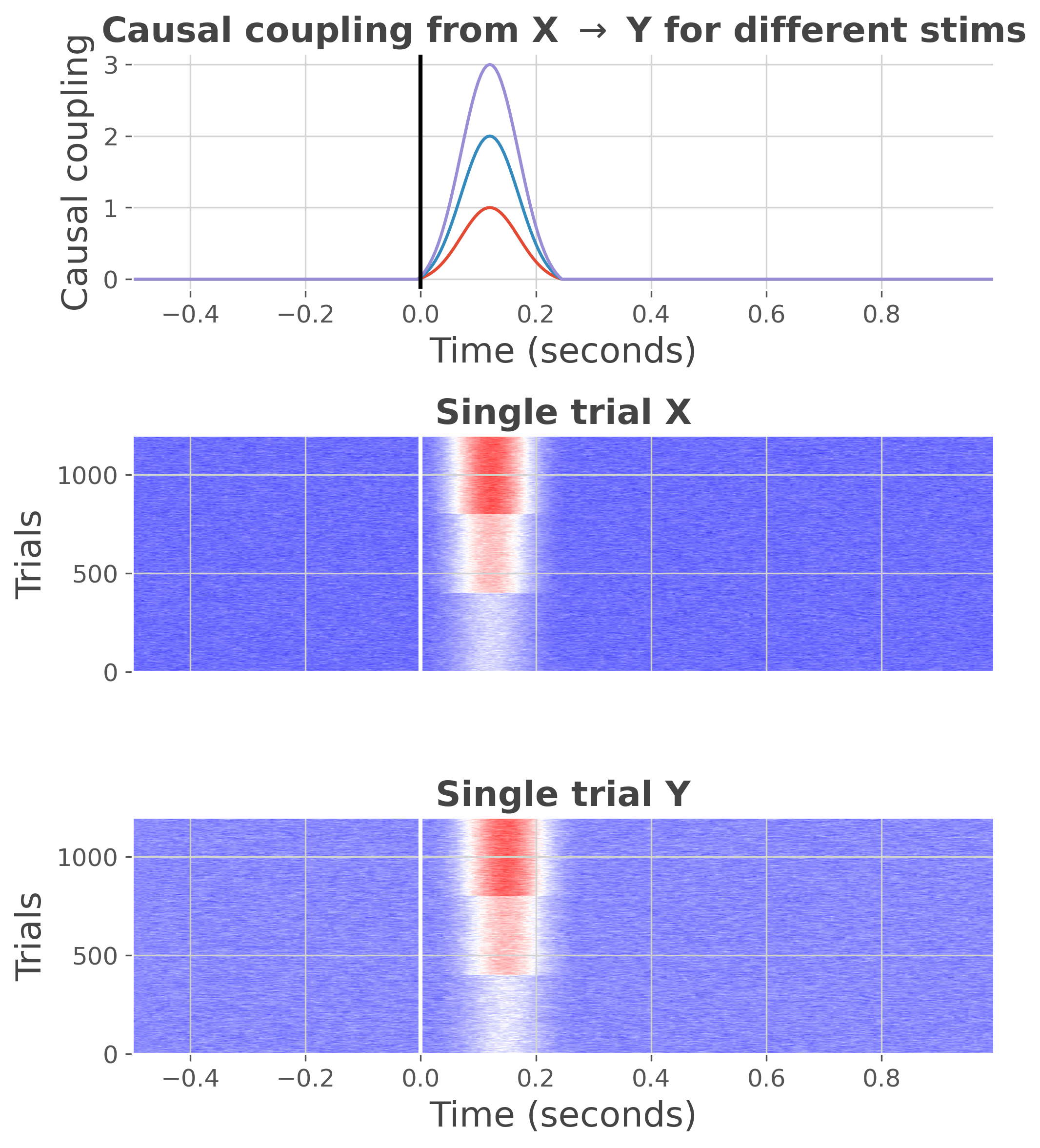
Data simulation

Here, we use an auto-regressive simulating a gamma increase.

net = False
avg_delay = False
ar_type = 'hga'
n_stim = 3
n_epochs = 400

ss = StimSpecAR()
ar = ss.fit(ar_type=ar_type, n_epochs=n_epochs, n_stim=n_stim, random_state=0)

print(ar)

plt.figure(figsize=(7, 8))
ss.plot(cmap='bwr')
plt.tight_layout()
plt.show()

<xarray.DataArray (trials: 1200, roi: 2, times: 300)>
array([[[ 0.3944541 ,  0.08947787,  0.21885247, ...,  0.15821295,
         -0.04185563,  0.07019032],
        [ 0.36321467, -0.13679289, -0.11810279, ...,  0.36246378,
         -0.15565568,  0.14413607]],

       [[-0.29214829,  0.37076929, -0.02642228, ..., -0.07226816,
         -0.22966976, -0.10883466],
        [ 0.46192319, -0.32896069, -0.18563208, ...,  0.1989966 ,
         -0.12743325,  0.30140249]],

       [[-0.34668654,  0.09331533, -0.21116721, ..., -0.37032276,
          0.46903415,  0.05036588],
        [-0.23992211,  0.11072083, -0.21288756, ..., -0.28649571,
         -0.07005528, -0.34033346]],

       ...,

       [[-0.01538188, -0.16898504,  0.23711941, ..., -0.01158757,
         -0.12814105, -0.06427391],
        [ 0.3718958 ,  0.09224002, -0.202277  , ..., -0.05967159,
         -0.47515636,  0.06669148]],

       [[ 0.2289687 ,  0.26491207, -0.28432468, ...,  0.44090788,
          0.19124113,  0.14904106],
        [ 0.18744301, -0.09694941,  0.39603464, ...,  0.05478838,
          0.18196749, -0.0345686 ]],

       [[-0.06437222, -0.23064244, -0.08996951, ...,  0.0400626 ,
          0.0977585 , -0.12655847],
        [ 0.04681595,  0.05029251,  0.1605935 , ...,  0.1253402 ,
          0.14925333, -0.22551455]]])
Coordinates:
  * trials   (trials) int64 1 1 1 1 1 1 1 1 1 1 1 1 ... 3 3 3 3 3 3 3 3 3 3 3 3
  * roi      (roi) <U1 'x' 'y'
  * times    (times) float64 -0.5 -0.495 -0.49 -0.485 ... 0.98 0.985 0.99 0.995
Attributes:
    n_stim:    3
    n_std:     3
    ar_type:   hga
    stimulus:  [1 2 3]

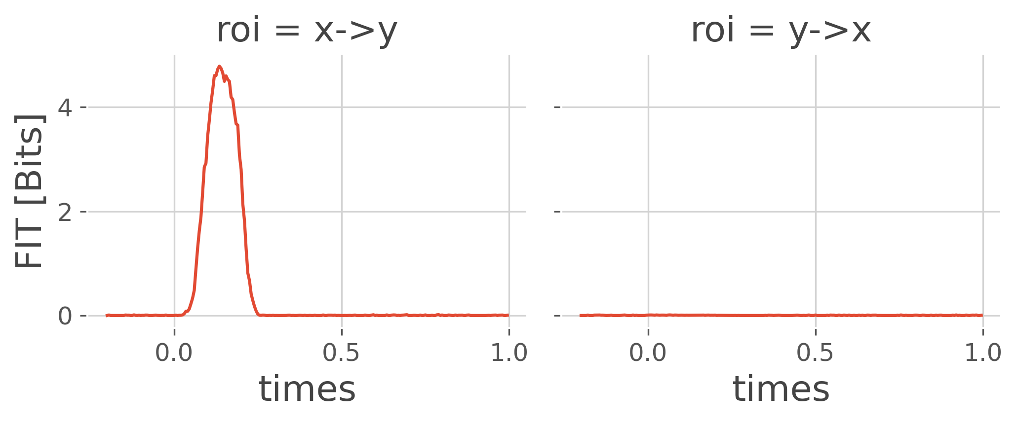
Compute Feature specific information transfer

Now we can use the simulated data to estimate the FIT.

# Compute the FIT

fit = conn_fit(ar, y='trials', roi='roi', times='times', mi_type='cd',
               max_delay=.3, net=net, verbose=False, avg_delay=avg_delay)

# Plot the results
fit.plot(x='times', col='roi')  # net = False

plt.show()

Estimated memory usage: 79 MB