Note
Go to the end to download the full example code.
Estimate comodulations between brain areas#
This example illustrates how to estimate the instantaneous comodulations using mutual information between pairwise ROI and also perform statistics.
import numpy as np
import xarray as xr

from itertools import product

from frites.simulations import sim_multi_suj_ephy
from frites.dataset import DatasetEphy
from frites.workflow import WfConnComod
from frites import set_mpl_style

import matplotlib.pyplot as plt
set_mpl_style()
Simulate electrophysiological data#
Let’s start by simulating MEG / EEG electrophysiological data coming from
multiple subjects using the function
frites.simulations.sim_multi_suj_ephy(). As a result, the x output
is a list of length n_subjects of arrays, each one with a shape of
n_epochs, n_sites, n_times
modality = 'meeg'
n_subjects = 5
n_epochs = 50
n_times = 100
x, roi, _ = sim_multi_suj_ephy(n_subjects=n_subjects, n_epochs=n_epochs,
                               n_times=n_times, modality=modality,
                               random_state=0, n_roi=4)
times = np.linspace(-1, 1, n_times)
Simulate spatial correlations#
Bellow, we start by simulating some distant correlations by injecting the activity of an ROI to another
for k in range(n_subjects):
x[k][:, [1], slice(20, 40)] += x[k][:, [0], slice(20, 40)]
x[k][:, [2], slice(60, 80)] += x[k][:, [3], slice(60, 80)]
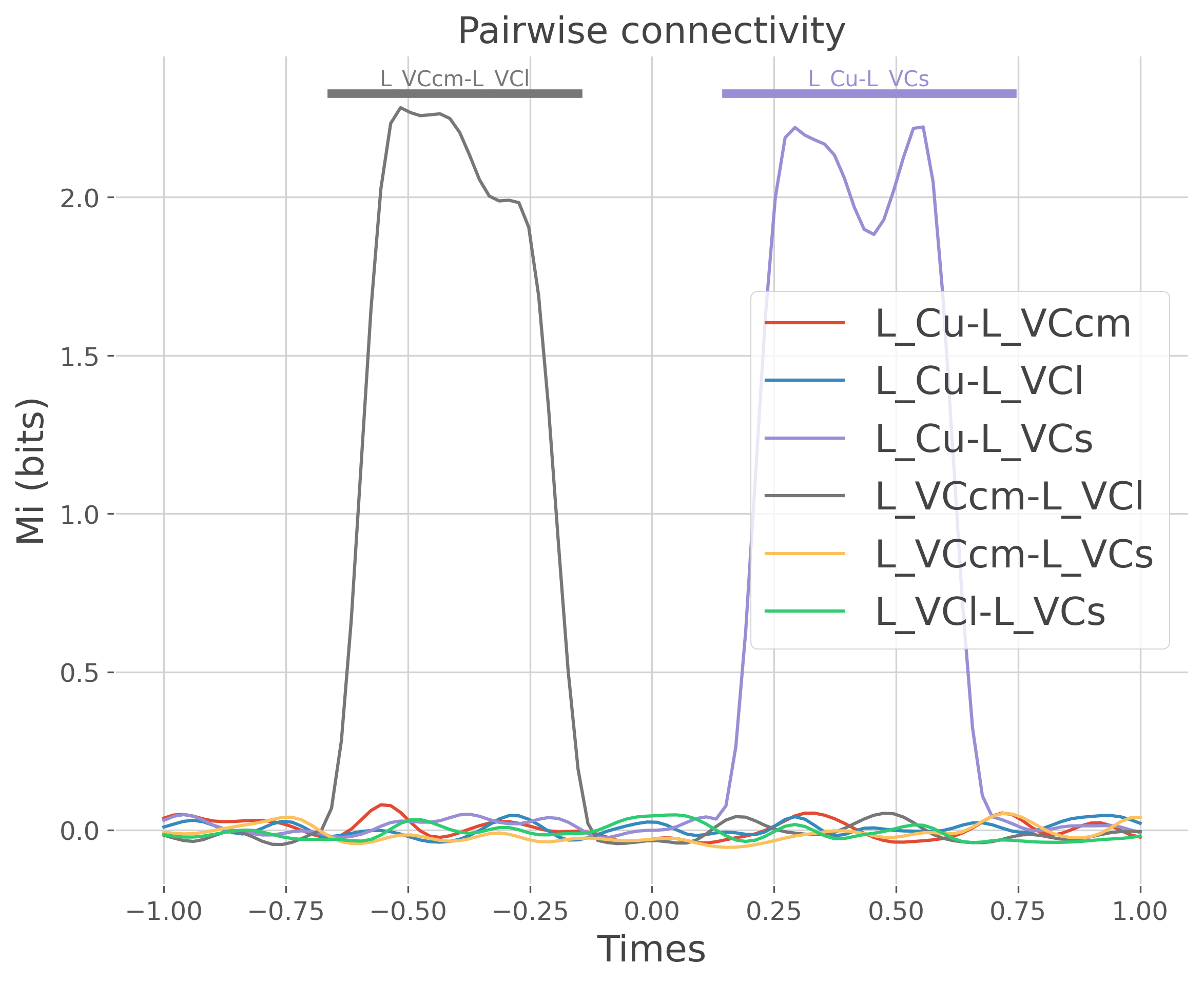
print(f'Corr 1 : {roi[0][0]}-{roi[0][1]} between [{times[20]}-{times[40]}]')
print(f'Corr 2 : {roi[0][2]}-{roi[0][3]} between [{times[60]}-{times[80]}]')
Corr 1 : L_VCcm-L_VCl between [-0.5959595959595959--0.19191919191919182]
Corr 2 : L_VCs-L_Cu between [0.21212121212121215-0.6161616161616164]
Define the electrophysiological dataset#
Now we define an instance of frites.dataset.DatasetEphy
dt = DatasetEphy(x, roi=roi, times=times)
Compute the pairwise connectivity#
Once we have the dataset instance, we can then define an instance of workflow
frites.workflow.WfConnComod. This instance is then used to compute
the pairwise connectivity
n_perm = 100  # number of permutations to compute
kernel = np.hanning(10)  # used for smoothing the MI

wf = WfConnComod(kernel=kernel)
mi, pv = wf.fit(dt, n_perm=n_perm, n_jobs=1)
print(mi)
  0%|          | Estimating MI : 0/6 [00:00<?,       ?it/s]
 17%|█▋        | Estimating MI : 1/6 [00:00<00:01,    4.21it/s]
 33%|███▎      | Estimating MI : 2/6 [00:00<00:00,    4.50it/s]
 50%|█████     | Estimating MI : 3/6 [00:00<00:00,    4.62it/s]
 67%|██████▋   | Estimating MI : 4/6 [00:00<00:00,    4.53it/s]
 83%|████████▎ | Estimating MI : 5/6 [00:01<00:00,    4.61it/s]
100%|██████████| Estimating MI : 6/6 [00:01<00:00,    4.57it/s]
100%|██████████| Estimating MI : 6/6 [00:01<00:00,    4.56it/s]
<xarray.DataArray 'mi' (times: 100, roi: 6)>
array([[ 3.81100170e-02,  9.93129635e-03,  3.08063622e-02,
        -1.57432552e-02, -6.46413969e-03, -1.42072425e-02],
       [ 4.78670422e-02,  1.91192336e-02,  4.39471590e-02,
        -2.48295685e-02, -9.89867658e-03, -1.90870444e-02],
       [ 4.97830695e-02,  2.78299595e-02,  4.91869950e-02,
        -3.27763185e-02, -1.17732336e-02, -2.18010919e-02],
       [ 4.42378373e-02,  3.11256639e-02,  4.41122743e-02,
        -3.54902207e-02, -1.09317976e-02, -2.17797055e-02],
       [ 3.54614078e-02,  2.64789554e-02,  3.09597577e-02,
        -2.97813754e-02, -7.22593180e-03, -1.87393195e-02],
       [ 2.90338318e-02,  1.55980511e-02,  1.60559750e-02,
        -1.82566072e-02, -1.28890639e-03, -1.36092876e-02],
       [ 2.67894121e-02,  2.79145887e-03,  5.40103015e-03,
        -7.51756587e-03,  4.73812172e-03, -7.90915604e-03],
       [ 2.73218532e-02, -7.89616349e-03, -4.27800566e-04,
        -3.53819107e-03,  1.00334736e-02, -2.98166005e-03],
       [ 2.92925541e-02, -1.18959045e-02, -5.27984078e-03,
        -8.68820963e-03,  1.53332565e-02,  1.78624950e-04],
       [ 3.08684130e-02, -6.19701377e-03, -1.09536592e-02,
        -2.09788897e-02,  2.03798908e-02, -5.68186008e-04],
...
       [-1.55322576e-02,  1.53093084e-02,  3.64898718e-03,
        -2.32618961e-02, -8.36461155e-03, -3.82575722e-02],
       [-1.05650033e-02,  2.72019144e-02,  1.00501854e-02,
        -2.81729709e-02, -1.86817089e-02, -3.83549006e-02],
       [ 9.97867229e-04,  3.59704840e-02,  1.34850531e-02,
        -2.89759278e-02, -2.33999399e-02, -3.72659062e-02],
       [ 1.34728115e-02,  4.05878562e-02,  1.38141548e-02,
        -2.61143734e-02, -2.40135389e-02, -3.54009462e-02],
       [ 2.24736359e-02,  4.33153684e-02,  1.36452655e-02,
        -2.08592129e-02, -2.04786052e-02, -3.27995353e-02],
       [ 2.33199680e-02,  4.57717725e-02,  1.41993169e-02,
        -1.39899823e-02, -1.00210812e-02, -2.99506386e-02],
       [ 1.45373274e-02,  4.63818215e-02,  1.44237465e-02,
        -7.83177679e-03,  7.41187732e-03, -2.79710396e-02],
       [-3.90368948e-04,  4.23275751e-02,  1.01411322e-02,
        -4.42294719e-03,  2.62532602e-02, -2.62370464e-02],
       [-1.45697842e-02,  3.34016522e-02,  9.98505930e-04,
        -3.72465911e-03,  3.88191796e-02, -2.33422674e-02],
       [-2.19995043e-02,  2.18230744e-02, -7.30826338e-03,
        -4.48774917e-03,  3.98892441e-02, -1.82330485e-02]])
Coordinates:
  * times    (times) float64 -1.0 -0.9798 -0.9596 -0.9394 ... 0.9596 0.9798 1.0
  * roi      (roi) <U12 'L_Cu-L_VCcm' 'L_Cu-L_VCl' ... 'L_VCl-L_VCs'
Attributes: (12/16)
    mi_type:         cc
    inference:       rfx
    kernel:          [0.         0.11697778 0.41317591 0.75       0.96984631 ...
    n_perm:          100
    random_state:    None
    ttest_pop_mean:  -0.00010172257964751625
    ...              ...
    mcp:             cluster
    tail:            1
    cluster_th:      None
    cluster_alpha:   0.05
    ttested:         0
    type:            mi
Plot the result of the DataArray#
# set to NaN everywhere it's not significant
is_signi = pv.data < .05
pv.data[~is_signi] = np.nan
pv.data[is_signi] = 1.02 * mi.data.max()

# plot each pair separately
plt.figure(figsize=(9, 7))
for n_r, r in enumerate(mi['roi'].data):
    # select the mi and p-values for the selected pair of roi
    mi_r, pv_r = mi.sel(roi=r), pv.sel(roi=r)
    plt.plot(times, mi_r, label=r, color=f"C{n_r}")
    if not np.isnan(pv_r.data).all():
        plt.plot(times, pv_r, color=f"C{n_r}", lw=4)
        x_txt = times[~np.isnan(pv_r)].mean()
        y_txt = 1.03 * mi.data.max()
        plt.text(x_txt, y_txt, r, color=f"C{n_r}", ha='center')
plt.legend()
plt.xlabel('Times')
plt.ylabel('Mi (bits)')
plt.title('Pairwise connectivity')
plt.show()
Total running time of the script: (0 minutes 3.793 seconds)
Estimated memory usage: 395 MB