PID: Decomposing the information carried by pairs of brain regions

This example illustrates how to decompose the information carried by pairs of brain regions about a behavioral variable y (e.g. stimulus, outcome, learning curve, etc.). Here, we use the Partial Information Decomposition (PID) that leads four non-negative and exclusive atoms of information: - The unique information carried by the first brain region about y - The unique information carried by the second brain region about y - The redundant information carried by both regions about y - The synergistic r complementary information carried by both regions about y

import numpy as np
import xarray as xr

from frites.simulations import StimSpecAR
from frites.conn import conn_pid

from frites import set_mpl_style

import matplotlib.pyplot as plt
set_mpl_style()

Data simulation

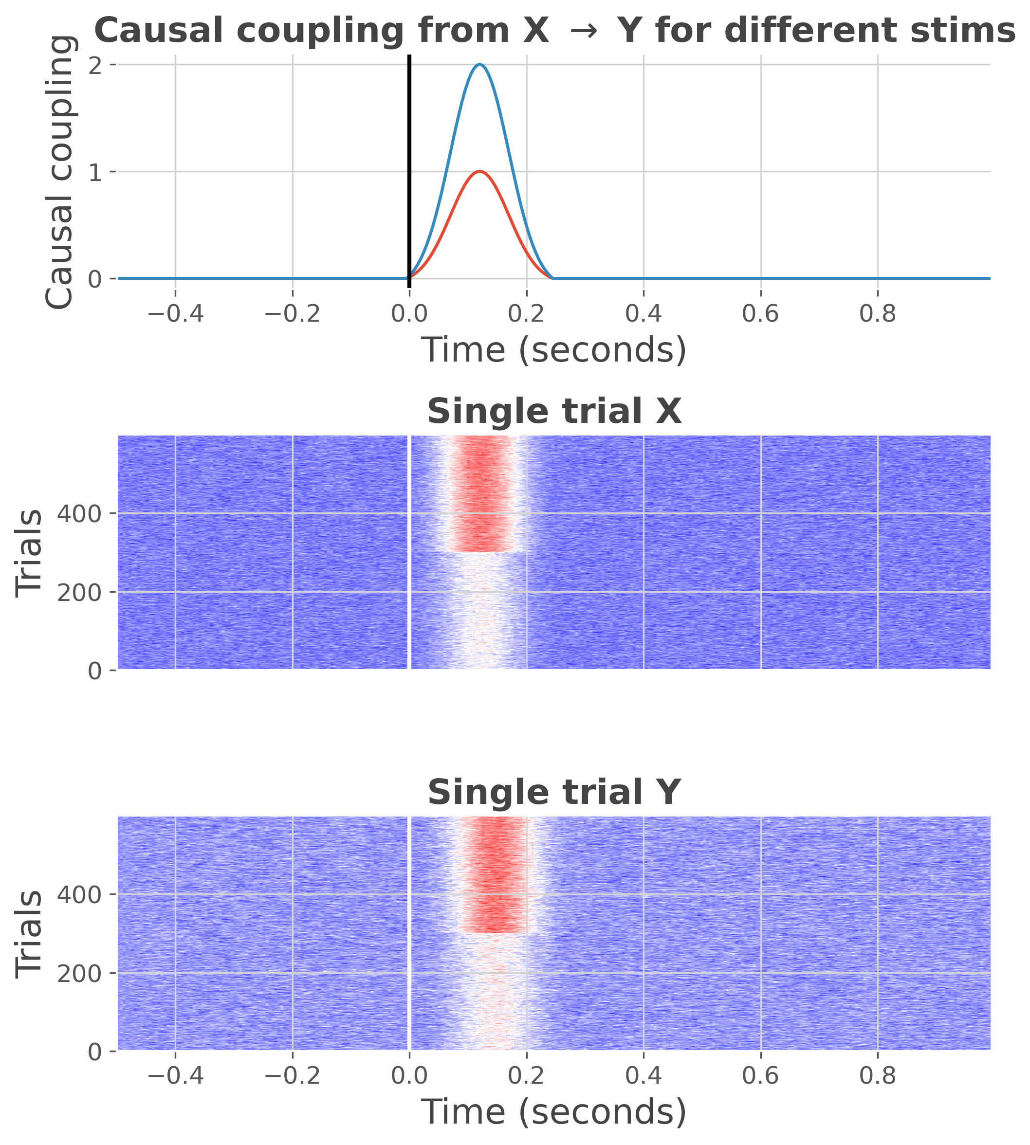
Let’s simulate some data. Here, we use an auto-regressive simulating a gamma increase. The gamma increase is modulated according to two conditions.

ar_type = 'hga'
n_stim = 2
n_epochs = 300

ss = StimSpecAR()
ar = ss.fit(ar_type=ar_type, n_epochs=n_epochs, n_stim=n_stim)

print(ar)

plt.figure(figsize=(7, 8))
ss.plot(cmap='bwr')
plt.tight_layout()
plt.show()

<xarray.DataArray (trials: 600, roi: 2, times: 300)>
array([[[ 0.15136261,  0.16723815, -0.20352514, ..., -0.3140514 ,
          0.28268379,  0.03006594],
        [ 0.23981999,  0.23954713, -0.07524559, ...,  0.24531103,
         -0.12692778, -0.33790791]],

       [[ 0.07782818,  0.11351779,  0.08816817, ..., -0.01267214,
         -0.25233664,  0.14371814],
        [ 0.31218496, -0.10861209, -0.55243616, ..., -0.15386609,
         -0.27610833, -0.12958128]],

       [[-0.09156302,  0.16527138,  0.07386311, ...,  0.16446816,
         -0.14523494, -0.03663393],
        [-0.02898154, -0.14533977,  0.22412981, ..., -0.04605822,
         -0.13451873, -0.4697649 ]],

       ...,

       [[ 0.23319511,  0.2276918 , -0.37713543, ..., -0.10780962,
         -0.3730847 , -0.54229869],
        [ 0.20385238, -0.18353852, -0.11485993, ...,  0.18995134,
          0.23485593, -0.19538096]],

       [[ 0.18108396,  0.12789712, -0.38841929, ..., -0.0488651 ,
          0.43939366, -0.17301611],
        [ 0.51243995,  0.00204005,  0.23204404, ..., -0.33951708,
          0.05367505, -0.34045041]],

       [[-0.03822738, -0.027729  ,  0.41268826, ..., -0.02783742,
         -0.18635673, -0.25233557],
        [-0.00389451, -0.02444377,  0.02582039, ...,  0.26486024,
         -0.03965586, -0.30082588]]])
Coordinates:
  * trials   (trials) int64 1 1 1 1 1 1 1 1 1 1 1 1 ... 2 2 2 2 2 2 2 2 2 2 2 2
  * roi      (roi) <U1 'x' 'y'
  * times    (times) float64 -0.5 -0.495 -0.49 -0.485 ... 0.98 0.985 0.99 0.995
Attributes:
    n_stim:    2
    n_std:     3
    ar_type:   hga
    stimulus:  [1 2]

Compute Partial Information Decomposition

Now we can use the simulated data to estimate the PID. Here, we’ll try to decompose at each time point, the information carried by pairs of brain regions about the two conditions.

# compute the PID
infotot, unique, redundancy, synergy = conn_pid(
    ar, 'trials', roi='roi', times='times', mi_type='cd', verbose=False
)

# plot the results
infotot.plot(color='C3', label=r"$Info_{Tot}$", linestyle='--')
redundancy.plot(color='C0', label=r"$Redundancy_{XY}$")
synergy.plot(color='C1', label=r"$Synergy_{XY}$")
unique.sel(roi='x').squeeze().plot(color='C4', label=r"$Unique_{X}$")
unique.sel(roi='y').squeeze().plot(color='C5', label=r"$Unique_{Y}$")
plt.legend()
plt.ylabel("Information [Bits]")
plt.axvline(0., color='C3', lw=2)
plt.title("Decomposition of the information carried by a pair of brain regions"
          "\nabout a task-related variable", fontweight='bold')
plt.show()

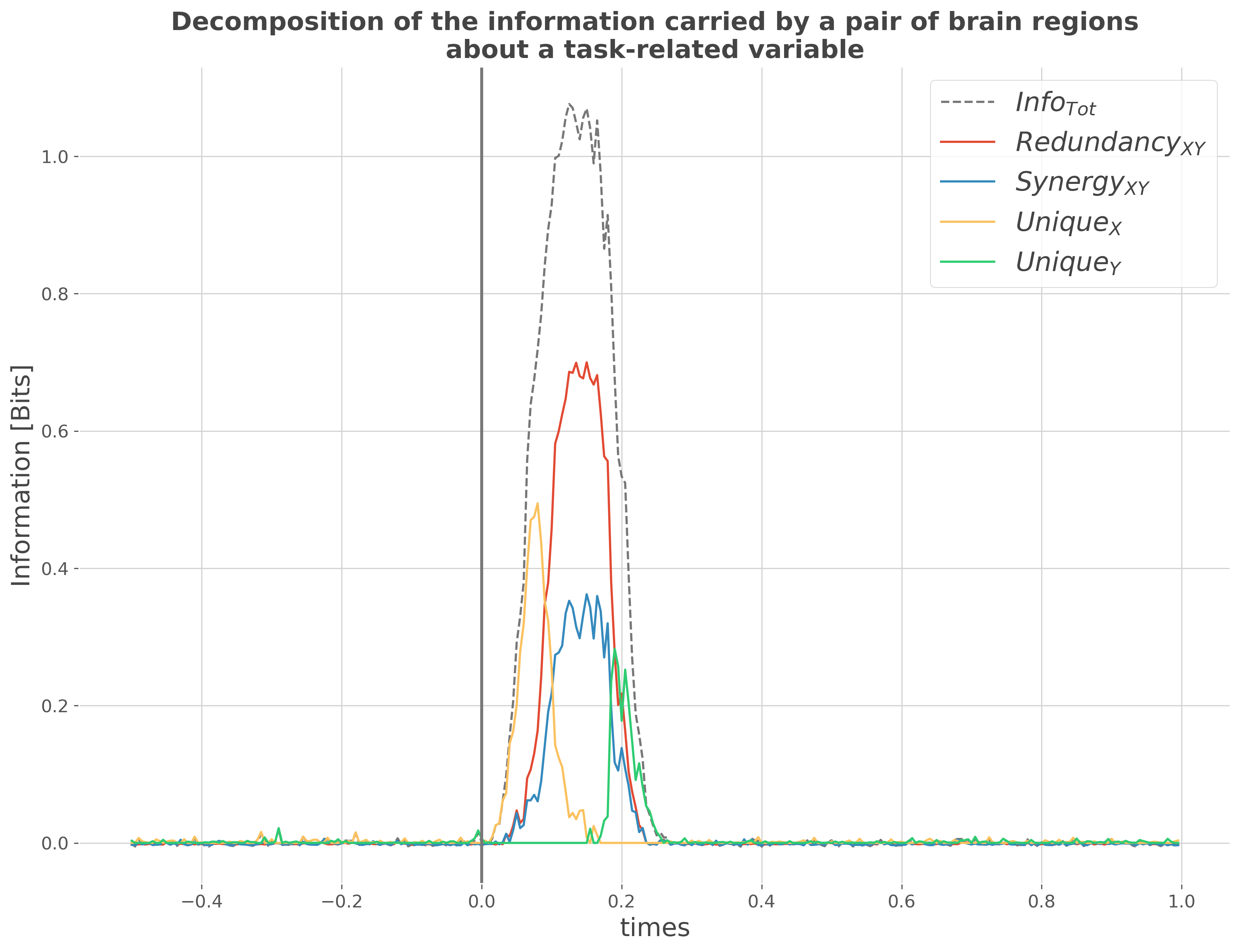
from the plot above, we can see that: 1. The total information carried by the pairs of regions (Info_{Tot}) 2. At the beginning, a large portion of the information is carried by the

first brain region (Unique_{X})

3. Then we can see a superimposition of redundancy (Redundancy_{XY}) and synergy (Synergy_{XY}) carried by both regions

4. Finally, later in time most of the information is carried by the second brain region Y (Unique_{X})

Estimated memory usage: 51 MB