Investigate relation of order

This example illustrates how to investigate whether the effect size between two conditions exceed the effect between two other conditions. To this end, we are first going to going the effect sizes inside the two conditions and then combine the effects (subtraction).

import numpy as np
import xarray as xr

from frites.simulations import sim_local_cd_ms
from frites.dataset import DatasetEphy
from frites.workflow import WfMi, WfMiCombine
from frites import set_mpl_style

import matplotlib.pyplot as plt
set_mpl_style()

Simulate electrophysiological data

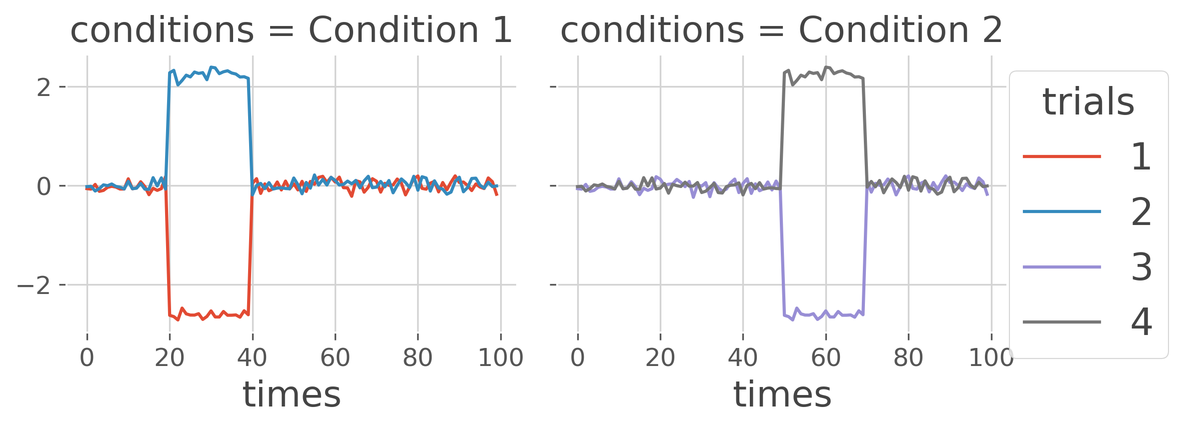
Let’s start by simulating MEG / EEG electrophysiological data coming from multiple subjects. We are going to be simulate two conditions : (i) in a first condition, we introduce some differences between two stimulus early in times (i.e. between time samples [20, 40]) and (ii) we introduce some differences between two other stimulus but this time, later in times (i.e. between time samples [50, 70])

n_epochs = 50
n_roi = 1
n_times = 100
n_subjects = 4
kw_data = dict(n_epochs=n_epochs, n_roi=n_roi)

def generate_data(cluster, condition=1):
    """Generate the data of a single condition."""
    remap = {
        1: {0: 1, 1: 2},
        2: {0: 3, 1: 4}
    }[condition]
    # generate data as standard arrays
    x, y, roi, times = sim_local_cd_ms(n_subjects, cl_index=cluster, **kw_data)
    # xarray conversion
    x_xr = []
    for k in range(n_subjects):
        _x = xr.DataArray(x[k], dims=('trials', 'roi', 'times'),
                          coords=([remap[k] for k in y[k]], roi[k], times))
        x_xr.append(_x)

    return x_xr

# generate the data of both conditions
x_1 = generate_data([20, 40], condition=1)  # stimulus {1, 2}
x_2 = generate_data([50, 70], condition=2)  # stimulus {3, 4}

# merge the two datasets (only for plotting the results)
x_1_plt = xr.concat(x_1, 'trials').groupby('trials').mean('trials')
x_2_plt = xr.concat(x_2, 'trials').groupby('trials').mean('trials')
x_12_plt = xr.Dataset({'Condition 1': x_1_plt, 'Condition 2': x_2_plt})
x_12_plt = x_12_plt.to_array('conditions')
x_12_plt.plot(x='times', hue='trials', col='conditions')
plt.show()

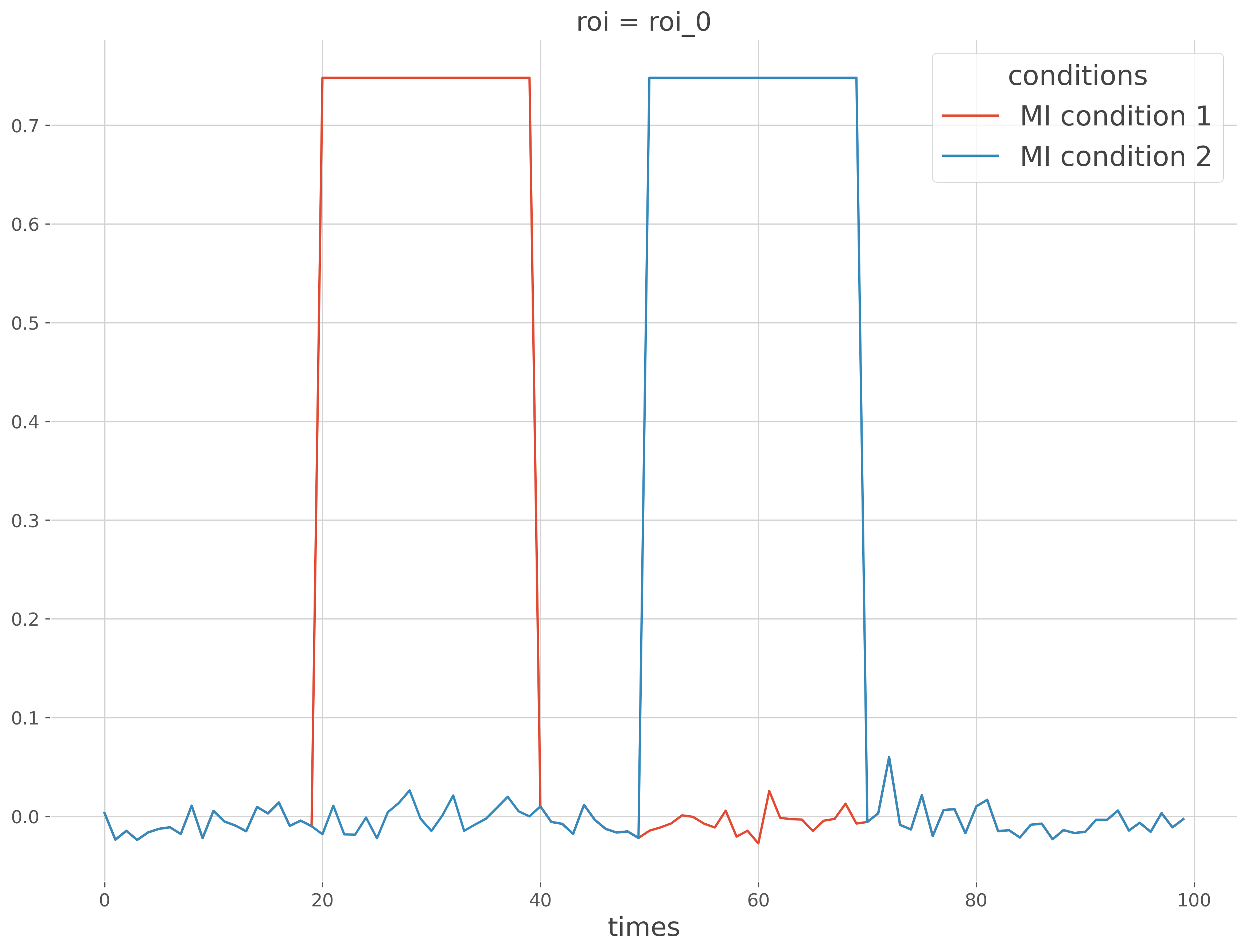
Compute effect size in both conditions

Now we can compute the effect size by means of mi in both conditions

# define additional arguments
kw_ds = dict(y='trials', roi='roi', times='times')
kw_wf = dict(inference='rfx', mi_type='cd')
kw_fit = dict(mcp='cluster', n_perm=200)

# define both electrophysiological datasets
ds_1 = DatasetEphy(x_1, **kw_ds)
ds_2 = DatasetEphy(x_2, **kw_ds)

# define two workflows of mutual-information
wf_1 = WfMi(**kw_wf)
wf_2 = WfMi(**kw_wf)

# compute effect size in both conditions
mi_1, pv_1 = wf_1.fit(ds_1, **kw_fit)
mi_2, pv_2 = wf_2.fit(ds_2, **kw_fit)

# merge mi of both conditions for plotting
mi_12 = xr.Dataset({
    'MI condition 1': mi_1.squeeze(),
    'MI condition 2': mi_2.squeeze()
}).to_array('conditions')
mi_12.plot(x='times', hue='conditions')
plt.show()

  0%|          | Estimating MI : 0/1 [00:00<?,       ?it/s]
100%|██████████| Estimating MI : 1/1 [00:01<00:00,    1.83s/it]
100%|██████████| Estimating MI : 1/1 [00:01<00:00,    1.83s/it]

  0%|          | Estimating MI : 0/1 [00:00<?,       ?it/s]
100%|██████████| Estimating MI : 1/1 [00:00<00:00,    4.24it/s]
100%|██████████| Estimating MI : 1/1 [00:00<00:00,    4.23it/s]

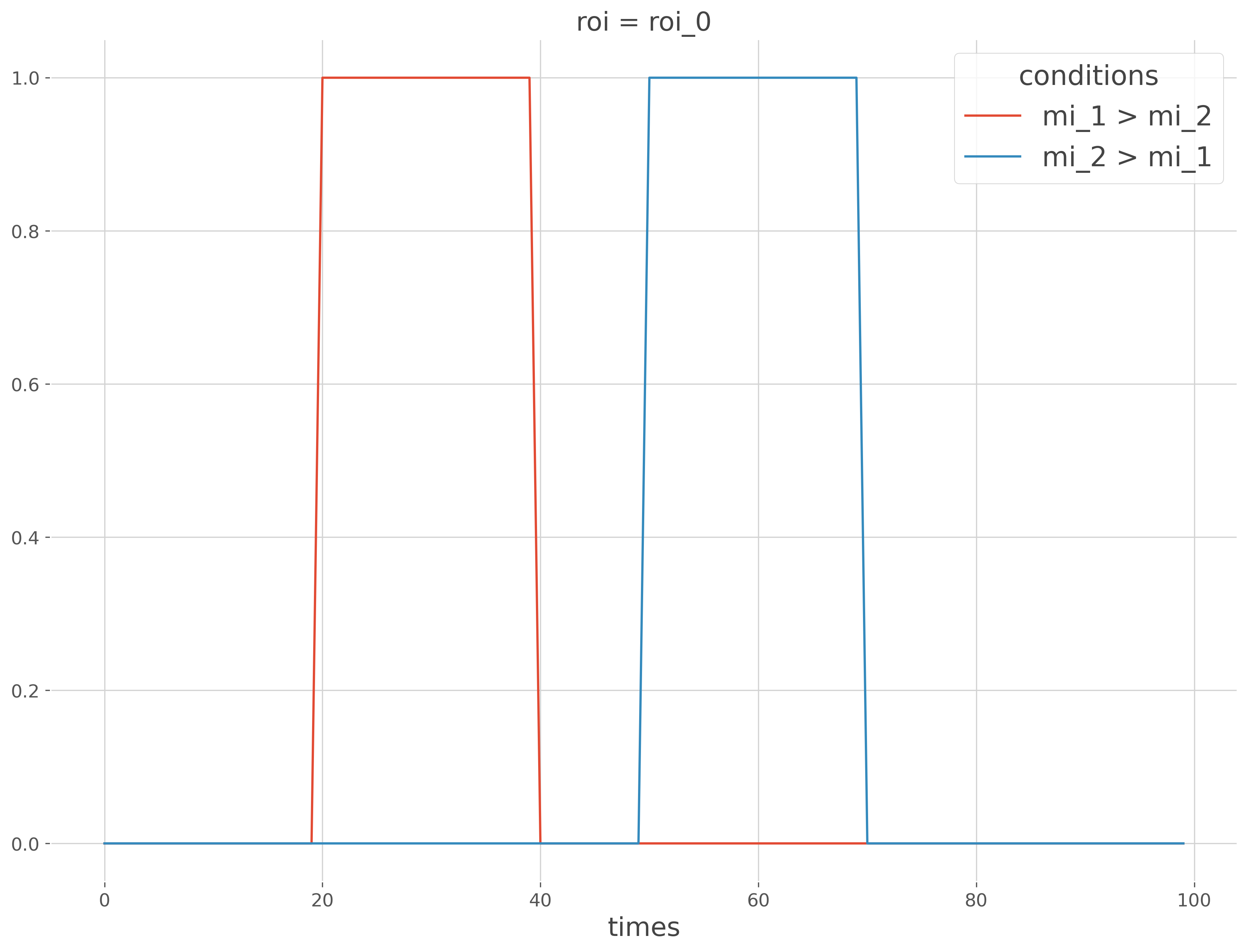
Investigate relation of order

Now we can investigate relations of order i.e. find everywhere the effect size in the first condition exceed the effect size of the second condition and conversely. To this end, we are going to combine the results of both workflows.

# find where mi_1 > mi_2
wf_12 = WfMiCombine(wf_1, wf_2)
mi_12, pv_12 = wf_12.fit(**kw_fit)

# find where mi_2 > mi_1
wf_21 = WfMiCombine(wf_2, wf_1)
mi_21, pv_21 = wf_21.fit(**kw_fit)

# combine the results for plotting
mi_order = xr.Dataset({
    'mi_1 > mi_2': (pv_12 < 0.05).squeeze(),
    'mi_2 > mi_1': (pv_21 < 0.05).squeeze(),
}).to_array('conditions')
mi_order.plot(x='times', hue='conditions')
plt.show()

Estimated memory usage: 76 MB