AR : simulate common driving input

This example illustrates an autoregressive model that simulates a common driving input (i.e X->Y and X->Z) and how it is measured using the covariance based Granger Causality

import numpy as np

from frites.simulations import StimSpecAR
from frites.conn import conn_covgc

import matplotlib.pyplot as plt

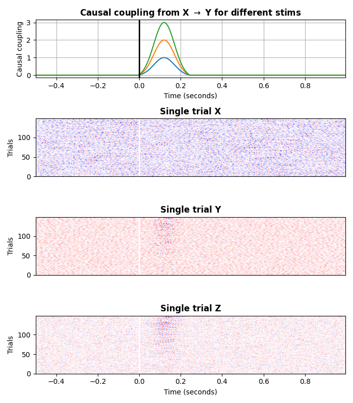
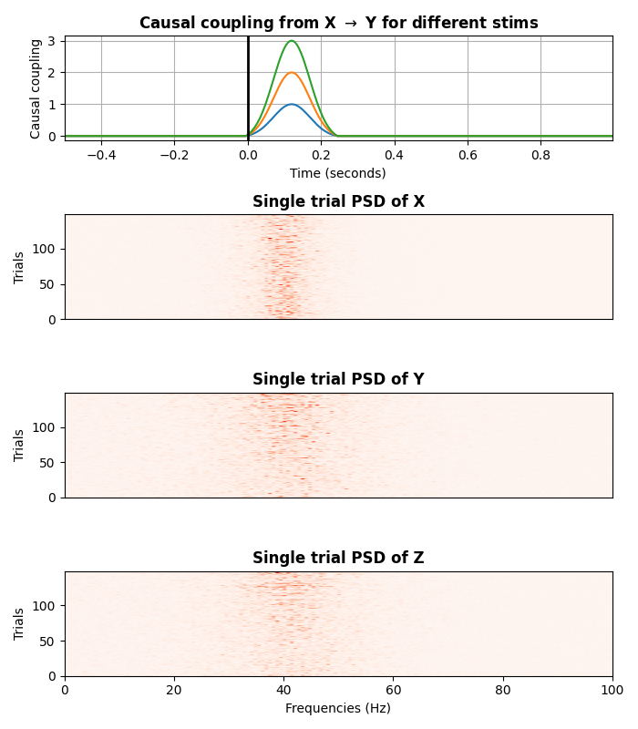
Simulate 3 nodes 40hz oscillations

Here, we use the class frites.simulations.StimSpecAR to simulate an stimulus-specific autoregressive model made of three nodes (X, Y and Z). This network simulates a transfer X->Y and X->Z. X is then called a common driving input for Y and Z

ar_type = 'osc_40_3'  # 40hz oscillations
n_stim = 3          # number of stimulus
n_epochs = 50       # number of epochs per stimulus

ss = StimSpecAR()
ar = ss.fit(ar_type=ar_type, n_epochs=n_epochs, n_stim=n_stim)
print(ar)

<xarray.DataArray (trials: 150, roi: 3, times: 300)>
array([[[ 0.25134439, -0.04588286, -0.38997855, ...,  0.47525239,
         -0.42996041, -0.35923828],
        [ 0.28807864,  0.32943226, -0.15219402, ...,  0.13200512,
          0.01481161,  0.18764986],
        [ 0.23625422,  0.16773289,  0.12441169, ...,  0.21856348,
         -0.46722405, -0.21981999]],

       [[-0.23425387,  0.2383734 ,  0.12571813, ...,  0.01028065,
          0.86762484,  0.64894575],
        [-0.00829905, -0.39008386,  0.08640293, ..., -0.17602529,
         -0.10660233, -0.25474297],
        [ 0.41032334,  0.10277509, -0.36499451, ..., -0.20049947,
         -0.44564005, -0.14311654]],

       [[-0.4885944 , -0.24088023,  0.5716417 , ...,  0.42614904,
          0.27062738, -0.17958764],
        [-0.35214581, -0.18335921, -0.04724976, ..., -0.00556085,
         -0.25871338, -0.35545094],
        [ 0.05442133, -0.08335093,  0.08436663, ..., -0.30889446,
         -0.3294228 ,  0.36430815]],
...
       [[ 0.33821833,  0.13736941, -0.04772936, ..., -0.12733071,
         -0.50344985, -0.06069676],
        [-0.35159565, -0.06081666,  0.41416986, ...,  0.43957058,
         -0.32255854, -0.14764446],
        [-0.13518498,  0.10178025,  0.32153082, ...,  0.23252699,
         -0.23642249,  0.07492754]],

       [[-0.19209026,  0.07261479,  0.11361513, ..., -0.25965606,
         -0.14892411,  0.10439557],
        [ 0.43026152, -0.02417257, -0.32028906, ...,  0.12009966,
          0.31882895,  0.14351507],
        [-0.1940527 , -0.06980799,  0.18732115, ..., -0.37826542,
         -0.36238163,  0.00259724]],

       [[ 0.19648887,  0.05398445, -0.14429047, ..., -0.37445137,
         -0.23278332,  0.33820427],
        [-0.0631801 , -0.0741364 , -0.11359434, ...,  0.05873906,
         -0.0372718 ,  0.13327158],
        [-0.10949838,  0.04815722,  0.04406834, ..., -0.03883177,
         -0.31380632, -0.14499861]]])
Coordinates:
  * trials   (trials) int64 1 1 1 1 1 1 1 1 1 1 1 1 ... 3 3 3 3 3 3 3 3 3 3 3 3
  * roi      (roi) <U1 'x' 'y' 'z'
  * times    (times) float64 -0.5 -0.495 -0.49 -0.485 ... 0.98 0.985 0.99 0.995
Attributes:
    n_stim:    3
    n_std:     3
    ar_type:   osc_40_3
    stimulus:  [1 2 3]

plot the network

plt.figure(figsize=(5, 4))
ss.plot_model()
plt.show()

plot the data

plt.figure(figsize=(7, 8))
ss.plot(cmap='bwr')
plt.tight_layout()
plt.show()

plot the power spectrum density (PSD)

plt.figure(figsize=(7, 8))
ss.plot(cmap='Reds', psd=True)
plt.tight_layout()
plt.show()

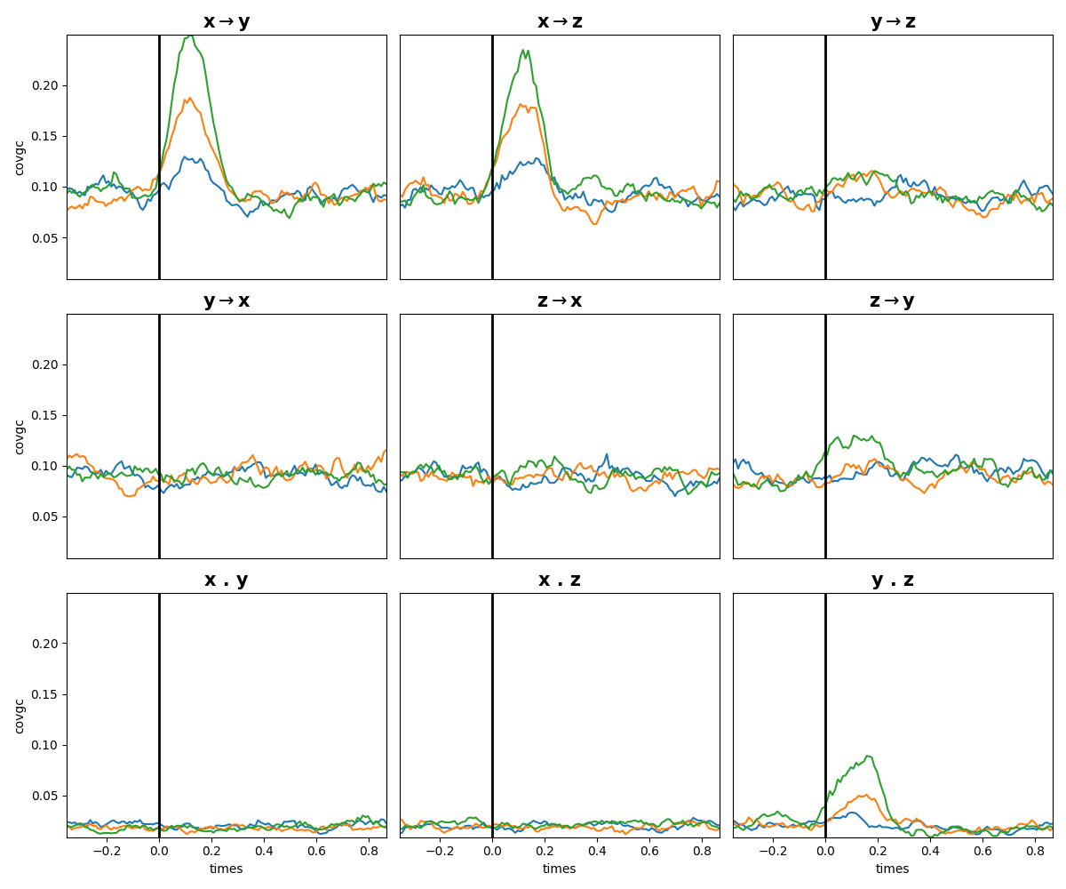
Compute the Granger-Causality

We then compute and plot the Granger Causality. From the plot you can see that there’s indeed an information transfer from X->Y and X->Z and, in addition, an instantaneous connectivity between Y.Z

dt = 50
lag = 5
step = 2
t0 = np.arange(lag, ar.shape[-1] - dt, step)
gc = conn_covgc(ar, roi='roi', times='times', dt=dt, lag=lag, t0=t0,
                n_jobs=-1)

# sphinx_gallery_thumbnail_number = 4
plt.figure(figsize=(12, 10))
ss.plot_covgc(gc)
plt.tight_layout()
plt.show()

  0%|          |  : 0/3 [00:00<?,       ?it/s]
100%|██████████|  : 3/3 [00:00<00:00, 1840.41it/s]

Estimated memory usage: 15 MB