Estimator comparison

This example compares implemented estimators for continuous variables.

import numpy as np
import pandas as pd

from frites.estimator import (GCMIEstimator, BinMIEstimator, CorrEstimator,
                              DcorrEstimator)
from frites import set_mpl_style

import matplotlib.pyplot as plt
from matplotlib.lines import Line2D
set_mpl_style()

Functions for data simulation

This first part contains functions used for simulating data.

def gen_mv_normal(n, cov):
    """Generate multi-variate normals."""
    sd = np.array([[1, cov], [cov, 1]])
    mean = np.array([0, 0])
    xy = np.random.multivariate_normal(mean, sd, size=n)
    xy += np.random.rand(*xy.shape) / 1000.
    x = xy[:, 0]
    y = xy[:, 1]
    return x, y


def rotate(xy, t):
    """Distribution rotation."""
    rot = np.array([[np.cos(t), np.sin(t)], [-np.sin(t), np.cos(t)]]).T
    return np.dot(xy, rot)


def generate_data(n, idx):
    """Generate simulated data."""
    x = np.linspace(-1, 1, n)
    mv_covs = [1.0, 0.8, 0.4, 0.0, -0.4, -0.8, -1.0]

    if idx in np.arange(7):  # multi-variate
        x, y = gen_mv_normal(n, mv_covs[idx])
        name = f'Multivariate (cov={mv_covs[idx]})'
        xlim = ylim = [-5, 5]
    elif idx == 7:  # curvy
        r = (np.random.random(n) * 2) - 1
        y = 4.0 * (x ** 2 - 0.5) ** 2 + (r / 3)
        name = 'Curvy'
        xlim, ylim = [-1, 1], [-1 / 3.0, 1 + (1 / 3.0)]
    if idx == 8:  # rotated uniform
        y = np.random.random(n) * 2 - 1
        xy = rotate(np.c_[x, y], -np.pi / 8.0)
        lim = np.sqrt(2 + np.sqrt(2)) / np.sqrt(2)
        x, y = xy[:, 0], xy[:, 1]
        name = 'Rotated uniform (1)'
        xlim = ylim = [-lim, lim]
    if idx == 9:  # rotated uniform
        y = np.random.random(n) * 2 - 1
        xy = rotate(np.c_[x, y], -np.pi / 4.0)
        lim = np.sqrt(2)
        x, y = xy[:, 0], xy[:, 1]
        name = 'Rotated uniform (2)'
        xlim = ylim = [-lim, lim]
    if idx == 10:  # smile
        r = (np.random.random(n) * 2) - 1
        y = 2 * (x ** 2) + r
        xlim, ylim = [-1, 1], [-1, 3]
        name = 'Smile'
    if idx == 11:  # mirrored smile
        r = np.random.random(n) / 2.0
        y = x ** 2 + r
        flipidx = np.random.permutation(len(y))[:int(n / 2)]
        y[flipidx] = -y[flipidx]
        name = 'Mirrored smile'
        xlim, ylim = [-1.5, 1.5], [-1.5, 1.5]
    if idx == 12:  # circle
        r = np.random.normal(0, 1 / 8.0, n)
        y = np.cos(x * np.pi) + r
        r = np.random.normal(0, 1 / 8.0, n)
        x = np.sin(x * np.pi) + r
        name = 'Circle'
        xlim, ylim = [-1.5, 1.5], [-1.5, 1.5]
    if idx == 13:  # 4 clusters
        sd = np.array([[1, 0], [0, 1]])
        xy1 = np.random.multivariate_normal([3, 3], sd, int(n / 4))
        xy2 = np.random.multivariate_normal([-3, 3], sd, int(n / 4))
        xy3 = np.random.multivariate_normal([-3, -3], sd, int(n / 4))
        xy4 = np.random.multivariate_normal([3, -3], sd, int(n / 4))
        xy = np.r_[xy1, xy2, xy3, xy4]
        x, y = xy[:, 0], xy[:, 1]
        name = '4 clusters'
        xlim = ylim = [-7, 7]

    return name, x, y, xlim, ylim

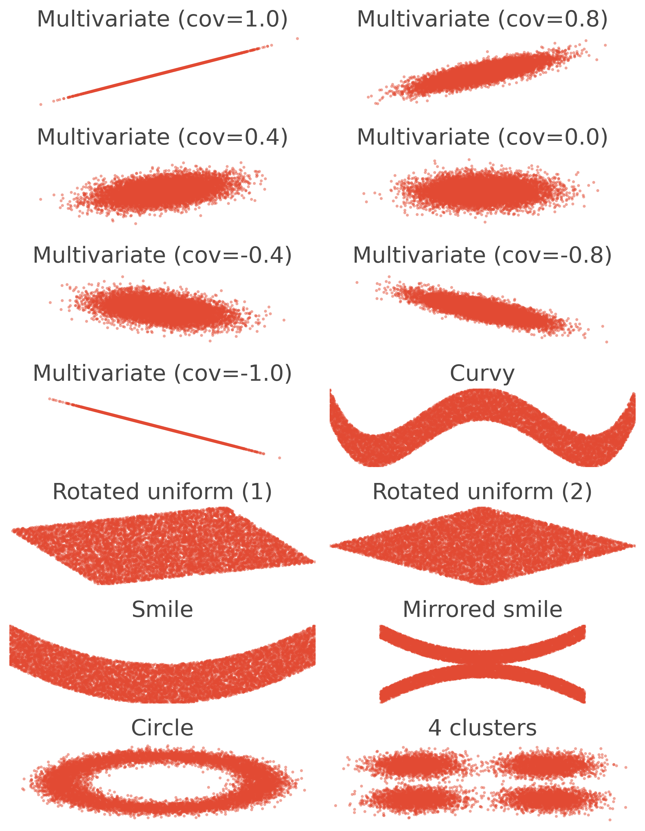
Plot the simulated data

In this section, we plot several scenarios of relation between a variable x and a variable y. The scenarios involve linear, non-linear, monotonic and non-monotonic relations.

# number of points
n = 10000

# plot the data
fig_data = plt.figure(figsize=(7, 9))
for i in range(14):
    name, x, y, xlim, ylim = generate_data(n, i)

    plt.subplot(7, 2, i + 1)
    ax = plt.gca()
    ax.scatter(x, y, s=5, edgecolors='none', alpha=.5)
    plt.xlim(xlim)
    plt.ylim(ylim)
    plt.title(name)
    ax.axis(False)

fig_data.tight_layout()
plt.show()

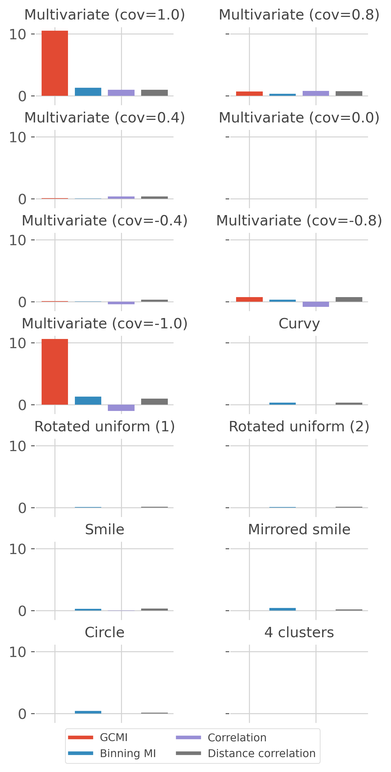
Computes information shared

In this final section, we compute the amount of information shared between the x and y variables using different estimators.

# define estimators
estimators = {
    'GCMI': GCMIEstimator(mi_type='cc', biascorrect=True),
    'Binning MI': BinMIEstimator(mi_type='cc'),
    'Correlation': CorrEstimator(),
    'Distance correlation': DcorrEstimator()
}


fig_info, axs = plt.subplots(
    nrows=7, ncols=2, sharex=True, sharey=True, figsize=(5, 9),
    gridspec_kw=dict(wspace=.4, hspace=.3, bottom=.05, top=.95, ))
axs = np.ravel(axs)

for i in range(14):
    name, x, y, _, _ = generate_data(n, i)

    ax = axs[i]
    plt.sca(ax)

    # computes information shared
    for n_e, (est_name, est) in enumerate(estimators.items()):
        info = float(est.estimate(x, y).squeeze())
        plt.bar(n_e, info, color=f"C{n_e}")

    ax.tick_params(axis='x', which='both', bottom=False, labelbottom=False)
    plt.title(name, fontsize=12)

# add the legend
plt.sca(axs[-2])
lines, names = [], []
for n_i, n in enumerate(estimators.keys()):
    lines.append(Line2D([0], [0], color=f"C{n_i}", lw=3))
    names.append(n)
plt.legend(lines, names, ncol=2, bbox_to_anchor=(.8, .05),
           fontsize=9, bbox_transform=fig_info.transFigure)

plt.show()

Estimated memory usage: 69 MB