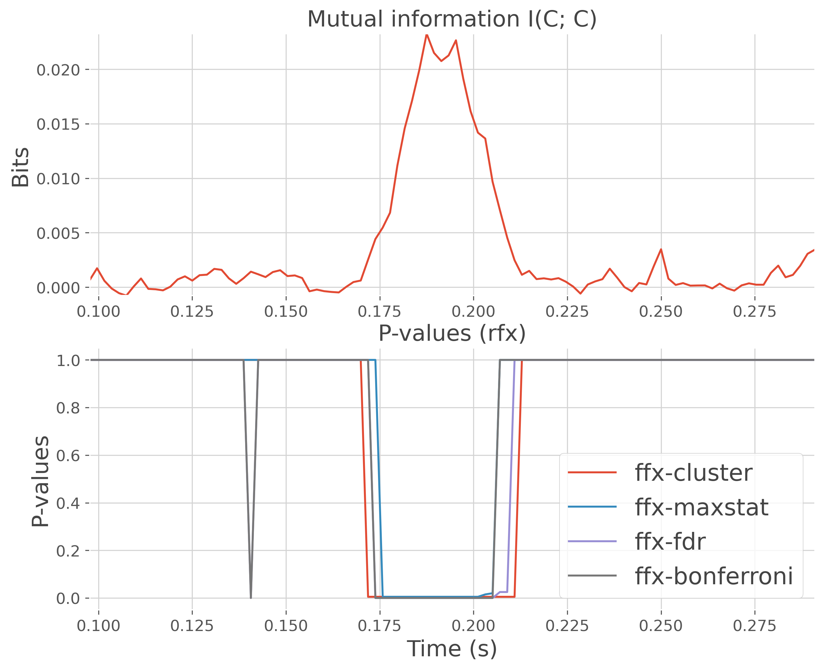
Compare between-subjects statistics when computing mutual information

This example illustrates how to define and run a workflow for computing mutual information and evaluate stastitics. Inference are made within-subjects (random effect = rfx).

import numpy as np

from frites.simulations import sim_multi_suj_ephy, sim_mi_cc
from frites.dataset import DatasetEphy
from frites.workflow import WfMi
from frites import set_mpl_style

import matplotlib.pyplot as plt
set_mpl_style()

Simulate electrophysiological data

Let’s start by simulating MEG / EEG electrophysiological data coming from multiple subjects using the function frites.simulations.sim_multi_suj_ephy(). As a result, the data output is a list of length n_subjects of arrays, each one with a shape of n_epochs, n_sites, n_times

modality = 'meeg'
n_subjects = 10
n_epochs = 400
n_times = 100
data, roi, time = sim_multi_suj_ephy(n_subjects=n_subjects, n_epochs=n_epochs,
                                     n_times=n_times, modality=modality,
                                     random_state=0)

Simulate mutual information

Once the data have been created, we simulate an increase of mutual information by creating a continuous variable y using the function frites.simulations.sim_mi_cc(). This allows to simulate model-based analysis by computing $I(data; y)$ where data and y are two continuous variables

y, _ = sim_mi_cc(data, snr=.1)

Create an electrophysiological dataset

Now, we use the frites.dataset.DatasetEphy in order to create a compatible electrophysiological dataset

dt = DatasetEphy(data, y=y, roi=roi, times=time, verbose=False)

Define the workflow

We now define the workflow for computing mi and evaluate statistics using the class frites.workflow.WfMi. Here, the type of mutual information to perform is ‘cc’ between it’s computed between two continuous variables. And we also specify the inference type ‘ffx’ for fixed-effect

mi_type = 'cc'
inference = 'rfx'
wf = WfMi(mi_type, inference, verbose=False)

Compute the mutual information and statistics

# list of corrections for multiple comparison
mcps = ['cluster', 'maxstat', 'fdr', 'bonferroni']
kw = dict(n_jobs=1, n_perm=200)
"""
The `cluster_th` input parameter specifies how the threshold is defined.
Use either :
* a float for a manual threshold
* None and it will be infered using the distribution of permutations
* 'tfce' for a TFCE threshold
"""
cluster_th = None  # {float, None, 'tfce'}

plt.figure(figsize=(10, 8))
for mcp in mcps:
    print(f'-> RFX / MCP={mcp}')
    mi, pvalues = wf.fit(dt, mcp=mcp, cluster_th=cluster_th, **kw)
    # remove p-values that exceed 0.05
    pvalues.data[pvalues >= .05] = 1.

    plt.subplot(212)
    plt.plot(time, pvalues.squeeze(), label=f'ffx-{mcp}')
    plt.xlabel('Time (s)'), plt.ylabel("P-values")
    plt.title("P-values (rfx)")
    plt.autoscale(tight=True, axis='x')
plt.legend()

plt.subplot(211)
plt.plot(time, mi.squeeze())
plt.ylabel("Bits")
plt.title("Mutual information I(C; C)")
plt.autoscale(tight=True)

plt.show()

-> RFX / MCP=cluster
-> RFX / MCP=maxstat
-> RFX / MCP=fdr
-> RFX / MCP=bonferroni

Estimated memory usage: 395 MB