MI between two continuous variables conditioned by a discret one

This example illustrates how to compute the mutual information between two continuous variables, conditioned by a discret one. The first variable is an electrophysiological data (M/EEG, intracranial). The second continuous is usually a regressor and the third is a discret variable composed with integers generally describing conditions. This type of mutual information is equivalent to partial correlation. For further details, see Ince et al., 2017 [12]

from frites.simulations import sim_multi_suj_ephy, sim_mi_ccd
from frites.dataset import DatasetEphy
from frites.workflow import WfMi
from frites import set_mpl_style

import matplotlib.pyplot as plt
set_mpl_style()

Simulate electrophysiological data

Let’s start by simulating MEG / EEG electrophysiological data coming from multiple subjects using the function frites.simulations.sim_multi_suj_ephy(). As a result, the x output is a list of length n_subjects of arrays, each one with a shape of n_epochs, n_sites, n_times

modality = 'meeg'
n_subjects = 5
n_epochs = 400
n_times = 100
x, roi, time = sim_multi_suj_ephy(n_subjects=n_subjects, n_epochs=n_epochs,
                                  n_times=n_times, modality=modality,
                                  random_state=0)

Extract the continuous and the discret variable

Here we extract the continuous and the discret variables from the random dataset generated above

y, z, _ = sim_mi_ccd(x, snr=1.)

Define the electrophysiological dataset

Now we define an instance of frites.dataset.DatasetEphy

dt = DatasetEphy(x, y=y, roi=roi, z=z, times=time)

Compute the mutual information

Once we have the dataset instance, we can then define an instance of workflow frites.workflow.WfMi. This instance is used to compute the mutual information

# mutual information type ('ccd' = continuous; continuous | discret)
mi_type = 'ccd'

# define the workflow
wf = WfMi(mi_type=mi_type)
# compute the mutual information
mi, _ = wf.fit(dt, mcp=None, n_jobs=1)

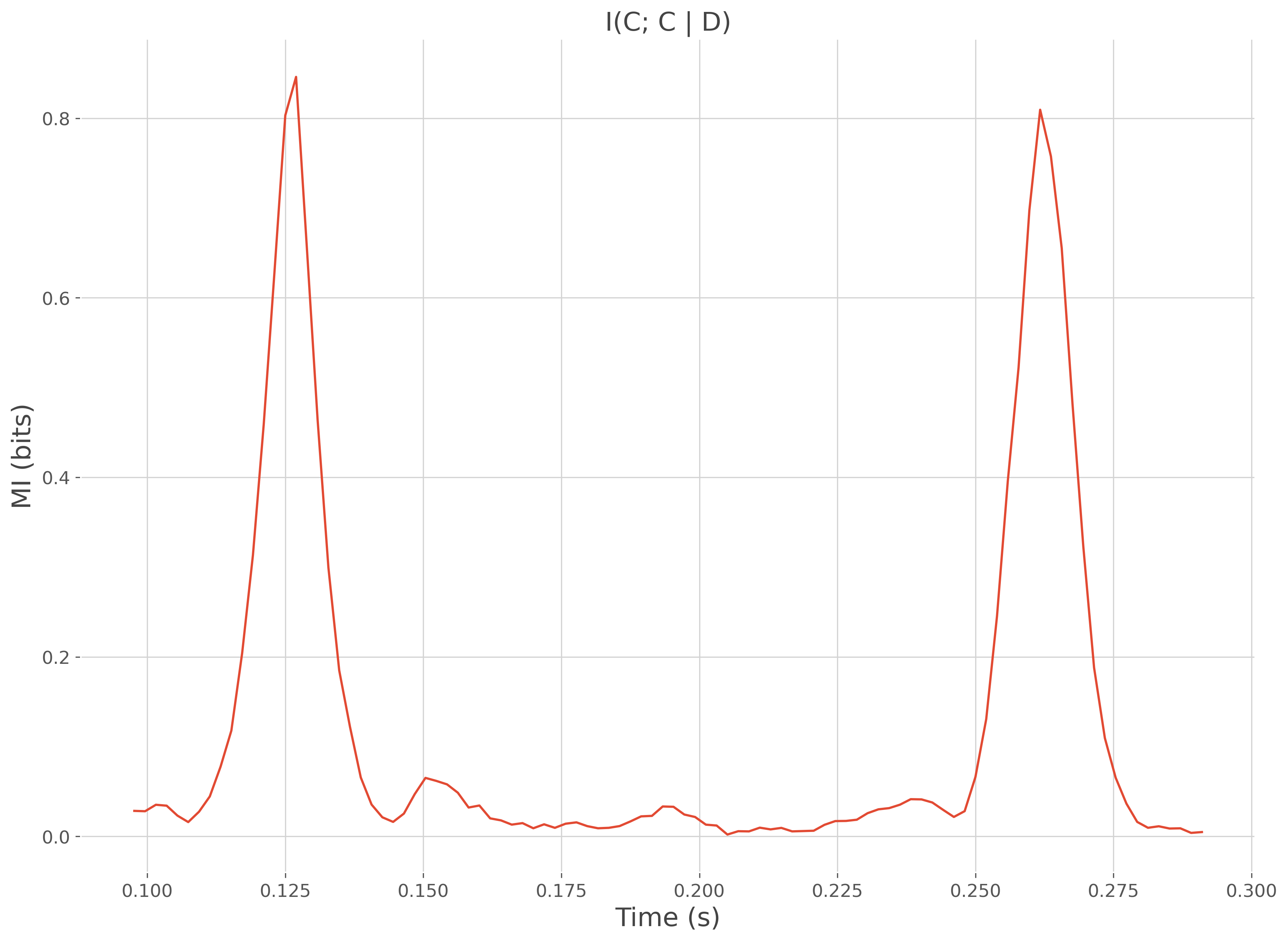
# plot the information shared between the data and the regressor y
plt.plot(time, mi)
plt.xlabel("Time (s)"), plt.ylabel("MI (bits)")
plt.title('I(C; C | D)')
plt.show()

  0%|          | Estimating MI : 0/1 [00:00<?,       ?it/s]
100%|██████████| Estimating MI : 1/1 [00:00<00:00,   12.00it/s]
100%|██████████| Estimating MI : 1/1 [00:00<00:00,   11.95it/s]

Estimated memory usage: 9 MB