Compute a conjunction analysis on mutual-information

In this example, we show how to perform a conjunction analysis which consist in getting the number of subjects that present significant effect.

import numpy as np

from frites.simulations import sim_single_suj_ephy
from frites.dataset import DatasetEphy
from frites.workflow import WfMi
from frites import set_mpl_style

import matplotlib.pyplot as plt
set_mpl_style()

Define where to put an effect for each subject

We start by organising where to set an affect for each subject. To this end, we define a dictionary where each key correspond to a subject. Then, for each subject we add the number of roi (n_roi), a color (color) and finally where to introduce effects ((roi_number, (effect_start, effect_end)))

n_epochs = 200
n_times = 100
ephy = {
    'subject_0': {
        'n_roi': 4,
        'color': 'red',
        'clusters': [(0, (10, 70)), (1, (30, 70)), (3, (50, 80))]
    },
    'subject_1': {
        'n_roi': 3,
        'color': 'green',
        'clusters': [(0, (50, 90)), (1, (30, 70)), (2, (20, 50))]
    },
    'subject_2': {
        'n_roi': 4,
        'color': 'blue',
        'clusters': [(0, (50, 90)), (2, (20, 50)), (3, (70, 90))]
    }
}
n_subjects = len(ephy)

Generate the electrophysiological data

Now we have all the properties where effect have to be present, we generate the electrophysiological data using the function frites.simulations.sim_single_suj_ephy().

# generate some random data
x, roi = [], []
for s_nb, s_name in enumerate(ephy.keys()):
    n_roi = ephy[s_name]['n_roi']
    _x, _roi, times = sim_single_suj_ephy(
        modality="meeg", sf=512., n_times=n_times, n_roi=n_roi,
        n_sites_per_roi=1, n_epochs=n_epochs, random_state=s_nb)
    x += [_x]
    roi += [np.array([f"roi_{k}" for k in range(n_roi)])]

# introduce an effect
y = []
for s_nb, s_name in enumerate(ephy.keys()):
    _y = np.random.normal(size=(n_epochs, 1))
    clusters = ephy[s_name]['clusters']

    for roi_nb, t_idx in clusters:
        x[s_nb][:, roi_nb, t_idx[0]:t_idx[1]] += _y

    y += [_y.squeeze()]

# Define the electrophysiological dataset
dt = DatasetEphy(x, y=y, roi=roi, times=times)

Compute the mutual information

Once we have the dataset instance, we can then define an instance of workflow frites.workflow.WfMi. This instance is used to compute the mutual information

# mutual information type ('cc' = continuous / continuous)
mi_type = 'cc'
inference = 'rfx'  # don't use 'ffx' for assessing conjunction analysis !

# define the workflow
wf = WfMi(mi_type)
# compute the mutual information
mi, pv = wf.fit(dt, mcp='cluster', n_perm=200, n_jobs=1, random_state=0)
n_roi = len(mi.roi.data)

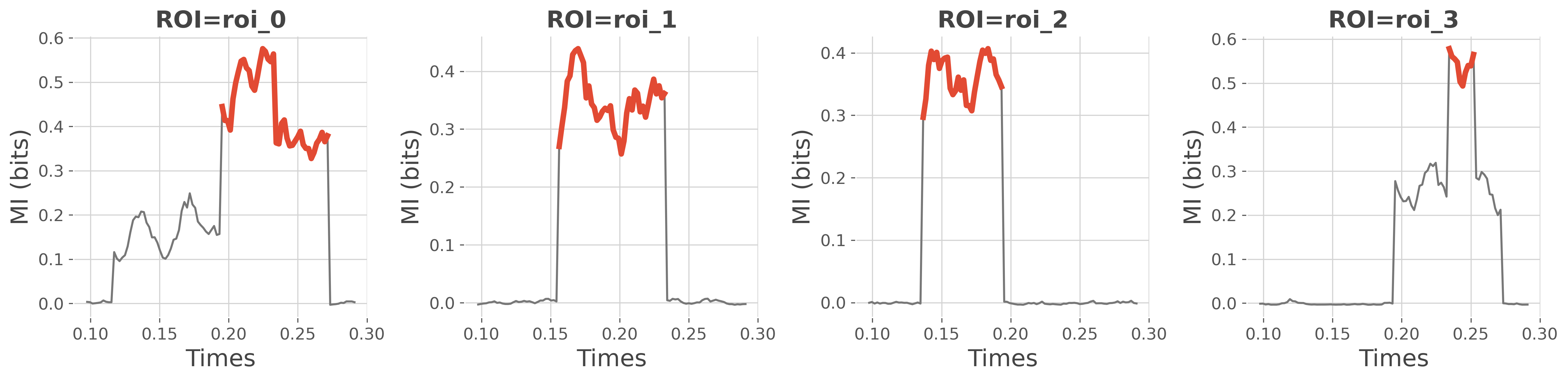
# plot where there's significant values of mi
fig = plt.figure(figsize=(16, 4))
for n_r, r in enumerate(mi.roi.data):
    # select the mi and p-values a specific roi
    mi_r, pv_r = mi.sel(roi=r), pv.sel(roi=r)
    # make a copy of the mi and set to nan everywhere it's not significant
    mi_sr = mi_r.copy()
    mi_sr.data[pv_r >= .05] = np.nan
    # superimpose mi and significant mi
    plt.subplot(1, n_roi, n_r + 1)
    plt.plot(times, mi_r, color='C3')
    plt.plot(times, mi_sr, lw=4, color='C0')
    plt.xlabel('Times'), plt.ylabel('MI (bits)')
    plt.title(f"ROI={r}", fontweight='bold')
plt.tight_layout()
plt.show()

  0%|          | Estimating MI : 0/4 [00:00<?,       ?it/s]
 25%|██▌       | Estimating MI : 1/4 [00:00<00:01,    1.60it/s]
 50%|█████     | Estimating MI : 2/4 [00:01<00:01,    1.61it/s]
 75%|███████▌  | Estimating MI : 3/4 [00:01<00:00,    1.62it/s]
100%|██████████| Estimating MI : 4/4 [00:02<00:00,    1.77it/s]
100%|██████████| Estimating MI : 4/4 [00:02<00:00,    1.76it/s]

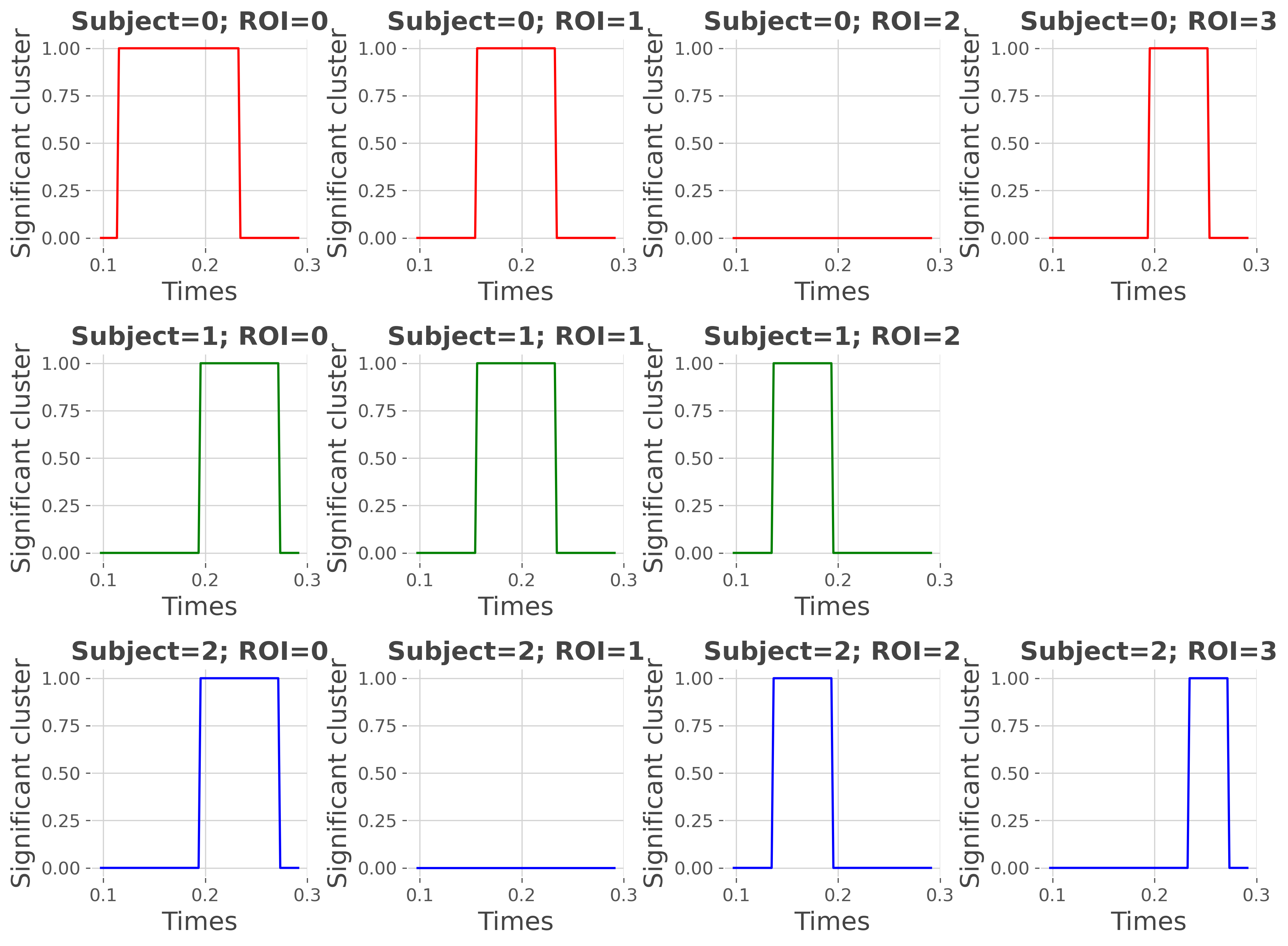
Perform the conjunction analysis

Now we have the values of MI we can compute the conjunction analysis. The following method returns two DataArray :

• conj_ssDataArray of shape (n_subjects, n_times, n_roi) that contains the

  significant MI of each subject

• conjDataArray of shape (n_times, n_roi) that contains the number of

  subjects that have a significant effect at each time point and for each roi

# perform the conjunction analysis
conj_ss, conj = wf.conjunction_analysis()

Plot where there’s significant effect for each subject

# printing the results
print(conj_ss)

fig = plt.figure(figsize=(12, 9))
q = 0
for n_s in range(n_subjects):
    color = ephy[f'subject_{n_s}']['color']
    for n_r, roi in enumerate(conj.roi.data):
        q += 1
        ss_data = conj_ss.sel(roi=roi, subject=n_s).T
        if np.isnan(ss_data).all():
            continue
        plt.subplot(n_subjects, n_roi, q)
        plt.plot(times, ss_data, color=color)
        plt.ylim(-0.05, 1.05)
        plt.title(f"Subject={n_s}; ROI={n_r}", fontweight='bold')
        plt.xlabel('Times'), plt.ylabel('Significant cluster')
plt.tight_layout()
plt.show()

<xarray.DataArray 'Single subject conjunction' (subject: 3, times: 100, roi: 4)>
array([[[ 0.,  0.,  0.,  0.],
        [ 0.,  0.,  0.,  0.],
        [ 0.,  0.,  0.,  0.],
        ...,
        [ 0.,  0.,  0.,  0.],
        [ 0.,  0.,  0.,  0.],
        [ 0.,  0.,  0.,  0.]],

       [[ 0.,  0.,  0., nan],
        [ 0.,  0.,  0., nan],
        [ 0.,  0.,  0., nan],
        ...,
        [ 0.,  0.,  0., nan],
        [ 0.,  0.,  0., nan],
        [ 0.,  0.,  0., nan]],

       [[ 0.,  0.,  0.,  0.],
        [ 0.,  0.,  0.,  0.],
        [ 0.,  0.,  0.,  0.],
        ...,
        [ 0.,  0.,  0.,  0.],
        [ 0.,  0.,  0.,  0.],
        [ 0.,  0.,  0.,  0.]]])
Coordinates:
  * times          (times) float64 0.09766 0.09961 0.1016 ... 0.2891 0.291
  * roi            (roi) <U5 'roi_0' 'roi_1' 'roi_2' 'roi_3'
  * subject        (subject) int64 0 1 2
    p              float64 0.05
    cluster_th     <U4 'none'
    cluster_alpha  float64 0.05
    mcp            <U7 'cluster'

Plot the number of subjects that have an effect

# printing the results
print(conj)

# sphinx_gallery_thumbnail_number = 2
fig = plt.figure(figsize=(18, 4))
for n_r, roi in enumerate(conj.roi.data):
    plt.subplot(1, n_roi, n_r + 1)
    plt.plot(times, conj.sel(roi=roi), lw=2)
    plt.title(f"ROI={roi}", fontweight='bold')
    plt.xlabel('Times'), plt.ylabel('# subjects')
    plt.ylim(-0.05, n_subjects + 0.05)
plt.tight_layout()
plt.show()

<xarray.DataArray 'Across subjects conjunction' (times: 100, roi: 4)>
array([[0., 0., 0., 0.],
       [0., 0., 0., 0.],
       [0., 0., 0., 0.],
       [0., 0., 0., 0.],
       [0., 0., 0., 0.],
       [0., 0., 0., 0.],
       [0., 0., 0., 0.],
       [0., 0., 0., 0.],
       [0., 0., 0., 0.],
       [1., 0., 0., 0.],
       [1., 0., 0., 0.],
       [1., 0., 0., 0.],
       [1., 0., 0., 0.],
       [1., 0., 0., 0.],
       [1., 0., 0., 0.],
       [1., 0., 0., 0.],
       [1., 0., 0., 0.],
       [1., 0., 0., 0.],
       [1., 0., 0., 0.],
       [1., 0., 0., 0.],
...
       [2., 0., 0., 1.],
       [2., 0., 0., 1.],
       [2., 0., 0., 1.],
       [2., 0., 0., 1.],
       [2., 0., 0., 1.],
       [2., 0., 0., 1.],
       [2., 0., 0., 1.],
       [2., 0., 0., 1.],
       [2., 0., 0., 1.],
       [2., 0., 0., 1.],
       [0., 0., 0., 0.],
       [0., 0., 0., 0.],
       [0., 0., 0., 0.],
       [0., 0., 0., 0.],
       [0., 0., 0., 0.],
       [0., 0., 0., 0.],
       [0., 0., 0., 0.],
       [0., 0., 0., 0.],
       [0., 0., 0., 0.],
       [0., 0., 0., 0.]])
Coordinates:
  * times          (times) float64 0.09766 0.09961 0.1016 ... 0.2891 0.291
  * roi            (roi) <U5 'roi_0' 'roi_1' 'roi_2' 'roi_3'
    p              float64 0.05
    cluster_th     <U4 'none'
    cluster_alpha  float64 0.05
    mcp            <U7 'cluster'

Estimated memory usage: 73 MB