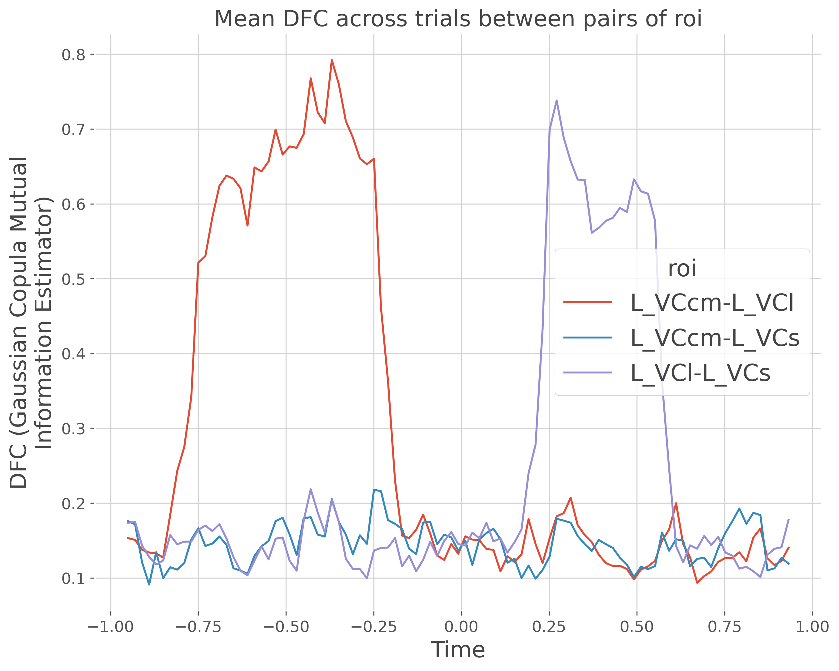
Estimate dynamic functional connectivity

This example illustrates how to compute the dynamic functional connectivity (DFC) using the mutual information (MI). This type of connectivity is computed for each trial either inside a single window or across multiple windows.

import numpy as np
from itertools import product

from frites.simulations import sim_single_suj_ephy
from frites.conn import conn_dfc, define_windows, plot_windows

from frites import set_mpl_style

import matplotlib.pyplot as plt
set_mpl_style()

Simulate electrophysiological data

Let’s start by simulating MEG / EEG electrophysiological data coming from a single subject. The output data of this single subject has a shape of (n_epochs, n_roi, n_times)

modality = 'meeg'
n_roi = 3
n_epochs = 50
n_times = 1000
x, roi, _ = sim_single_suj_ephy(n_epochs=n_epochs, n_times=n_times,
                                modality=modality, n_roi=n_roi, random_state=0)
times = np.linspace(-1, 1, n_times)

Simulate spatial correlations

Bellow, we are simulating some distant correlations by injecting the activity of an ROI to another

x[:, [1], slice(100, 400)] += x[:, [0], slice(100, 400)]
x[:, [2], slice(600, 800)] += x[:, [1], slice(600, 800)]
print(f'Corr 1 : {roi[0]}-{roi[1]} between [{times[100]}-{times[400]}]')
print(f'Corr 2 : {roi[2]}-{roi[1]} between [{times[600]}-{times[800]}]')

Corr 1 : L_VCcm-L_VCl between [-0.7997997997997999--0.19919919919919926]
Corr 2 : L_VCs-L_VCl between [0.20120120120120122-0.6016016016016015]

Define sliding windows

Next, we define, and plot sliding windows in order to compute the DFC on consecutive time windows. In this example we used windows of length 100ms and 5ms between each consecutive windows

slwin_len = .1    # 100ms window length
slwin_step = .02  # 20ms between consecutive windows
win_sample = define_windows(times, slwin_len=slwin_len,
                            slwin_step=slwin_step)[0]
times_p = times[win_sample].mean(1)

# plt.figure(figsize=(10, 8))
# plot_windows(times, win_sample, title='Sliding windows')
# plt.ylim(-1, 1)
# plt.show()

Compute the DFC

The DFC is going to be computed per trials, bewteen pairs of ROI and inside each of the temporal window

# compute DFC
dfc = conn_dfc(x, win_sample, times=times, roi=roi, n_jobs=1)
print(dfc)

plt.figure(figsize=(10, 8))
# plt.plot(times_p, dfc.mean('trials').T)
dfc.mean('trials').plot.line(x='times', hue='roi')
plt.xlabel('Time')
plt.title("Mean DFC across trials between pairs of roi")
plt.show()

  0%|          | Estimating DFC : 0/3 [00:00<?,       ?it/s]
 67%|██████▋   | Estimating DFC : 2/3 [00:00<00:00,   78.05it/s]
100%|██████████| Estimating DFC : 3/3 [00:00<00:00,   78.70it/s]
<xarray.DataArray 'DFC (Gaussian Copula Mutual Information Estimator)' (
                                                                        trials: 50,
                                                                        roi: 3,
                                                                        times: 95)>
array([[[4.74126835e-04, 4.86970457e-05, 1.15753941e-01, ...,
         1.44106135e-01, 1.00405946e-01, 8.37376192e-02],
        [3.29334080e-01, 3.09351981e-01, 7.13511854e-02, ...,
         6.81263686e-04, 2.51765386e-03, 3.19818184e-02],
        [9.04738065e-03, 2.04119571e-02, 2.55241338e-02, ...,
         6.54823380e-03, 1.80942327e-01, 7.69555792e-02]],

       [[2.43588135e-01, 4.48731631e-02, 3.06968745e-02, ...,
         1.19652078e-02, 1.41519258e-05, 1.56958587e-02],
        [1.19740553e-01, 4.07272950e-02, 1.60232615e-02, ...,
         4.46936190e-02, 5.86355664e-02, 7.60393683e-04],
        [1.73070922e-01, 1.90565914e-01, 3.83086987e-02, ...,
         1.16546720e-01, 1.21132061e-01, 3.26294273e-01]],

       [[3.59413236e-01, 6.76742554e-01, 8.00896406e-01, ...,
         2.62994856e-01, 3.78555506e-01, 3.44151706e-01],
        [6.52924832e-03, 1.69114739e-01, 2.32962683e-01, ...,
         2.62315989e-01, 3.79843652e-01, 1.67509735e-01],
        [8.95062694e-04, 4.41071056e-02, 2.38820821e-01, ...,
         2.81423610e-02, 7.95110539e-02, 4.08294201e-01]],
...
       [[2.07532123e-02, 3.34448464e-06, 3.19930399e-03, ...,
         2.95763791e-01, 1.60798971e-02, 1.35861740e-01],
        [6.86131716e-01, 4.58753556e-01, 1.49167523e-01, ...,
         3.07976492e-02, 1.27379432e-01, 6.57524914e-02],
        [1.18787738e-03, 4.60020150e-04, 3.37673649e-02, ...,
         2.37936508e-02, 1.87671706e-01, 1.34078279e-01]],

       [[7.02991262e-02, 7.39582926e-02, 3.76868337e-01, ...,
         1.00256223e-02, 2.14382401e-03, 1.74317230e-02],
        [1.44385636e-01, 1.77252650e-01, 2.52936292e-03, ...,
         2.17671096e-02, 1.07206358e-02, 2.39495244e-02],
        [8.77984054e-03, 1.95415434e-03, 1.42009801e-03, ...,
         3.53378356e-01, 3.31914216e-01, 4.86238658e-01]],

       [[6.26457098e-04, 6.44705370e-02, 4.74612694e-03, ...,
         5.78350900e-03, 7.82634515e-07, 6.35968670e-02],
        [6.88552320e-01, 6.04924738e-01, 5.80820143e-02, ...,
         7.78488629e-03, 6.61413297e-02, 2.66898096e-01],
        [4.23928313e-02, 8.31796043e-03, 1.45379873e-02, ...,
         1.08158283e-01, 9.71827563e-03, 2.18945459e-01]]])
Coordinates:
  * trials   (trials) int64 0 1 2 3 4 5 6 7 8 9 ... 41 42 43 44 45 46 47 48 49
  * roi      (roi) <U12 'L_VCcm-L_VCl' 'L_VCcm-L_VCs' 'L_VCl-L_VCs'
  * times    (times) float64 -0.9499 -0.9299 -0.9099 ... 0.8919 0.9119 0.9319
Attributes:
    win_sample:  [  0  50  10  60  20  70  30  80  40  90  50 100  60 110  70...
    win_times:   [-0.94994995 -0.92992993 -0.90990991 -0.88988989 -0.86986987...
    agg_ch:      0
    type:        dfc
    estimator:   Gaussian Copula Mutual Information Estimator
    unit:        Bits
    sfreq:       499.50000000001125
    sources:     [0, 0, 1]
    targets:     [1, 2, 2]

Estimated memory usage: 9 MB