AR : pairwise illustration#

This example illustrates a simple autoregressive model simulating a stimulus-specific information transfer from a source X to a target Y.

from frites import set_mpl_style
from frites.simulations import StimSpecAR

import matplotlib.pyplot as plt
set_mpl_style()

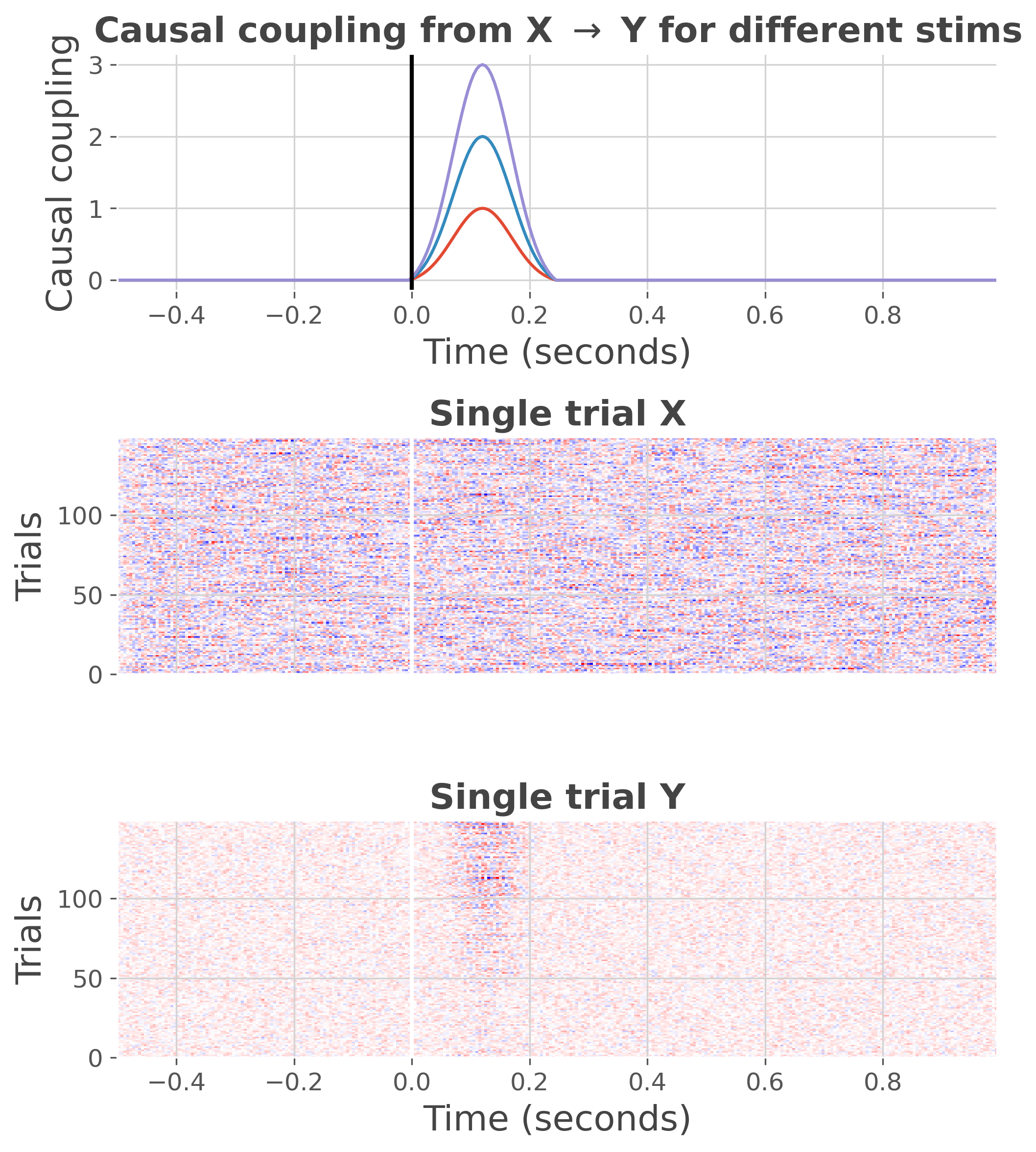
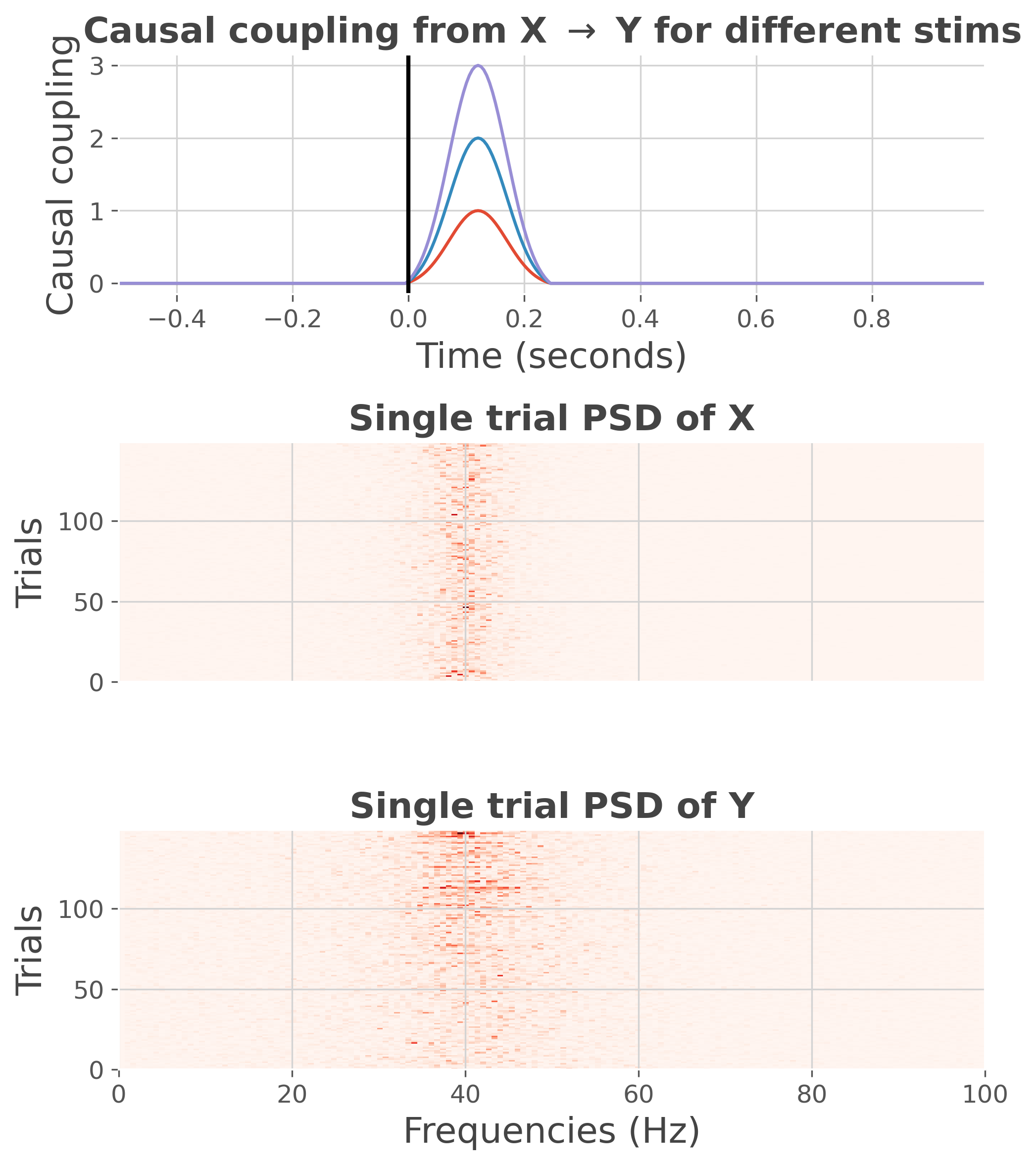
Simulate 40hz oscillations#

Here, we use the class frites.simulations.StimSpecAR to simulate an stimulus-specific autoregressive model. For the pairwise models, you can choose :

‘hga’ : high-gamma burst

‘osc_40’ / ‘osc_20’ : respectivelly 20hz and 40hz oscillations

‘ding_2’ : pairwise Ding’s model [7]

ar_type = 'osc_40'  # 40hz oscillations
n_stim = 3          # number of stimulus
n_epochs = 50       # number of epochs per stimulus

ss = StimSpecAR()
ar = ss.fit(ar_type=ar_type, n_epochs=n_epochs, n_stim=n_stim)

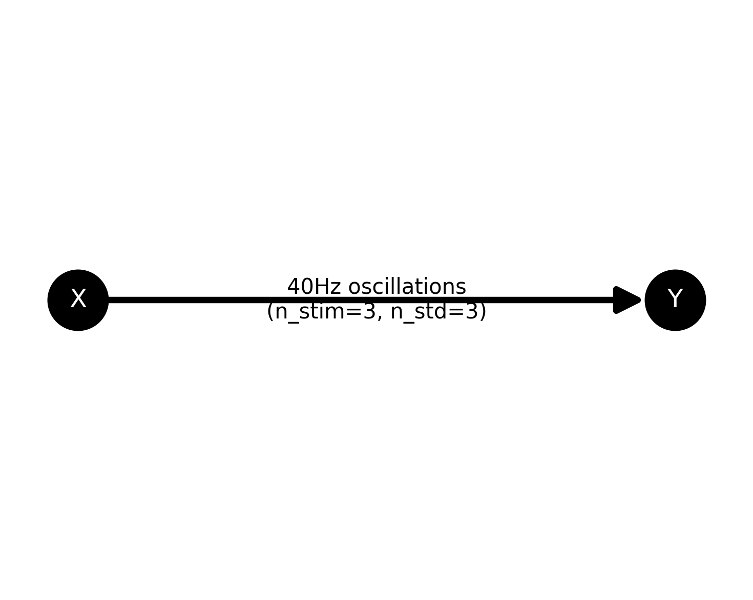
plot the network

plt.figure(figsize=(5, 4))
ss.plot_model()
plt.show()

plot the data

plt.figure(figsize=(7, 8))
ss.plot(cmap='bwr')
plt.tight_layout()
plt.show()

$Causal coupling from X $\rightarrow$ Y for different stims, Single trial X, Single trial Y$

plot the power spectrum density (PSD)

plt.figure(figsize=(7, 8))
ss.plot(cmap='Reds', psd=True)
plt.tight_layout()
plt.show()

$Causal coupling from X $\rightarrow$ Y for different stims, Single trial PSD of X, Single trial PSD of Y$

Total running time of the script: (0 minutes 2.906 seconds)

Estimated memory usage: 63 MB

Gallery generated by Sphinx-Gallery