Note
Go to the end to download the full example code.
Estimate the empirical confidence interval#
This example illustrates how to estimate the confidence interval
import numpy as np

from frites.simulations import sim_local_cc_ms
from frites.dataset import DatasetEphy
from frites.workflow import WfMi
from frites import set_mpl_style

import matplotlib.pyplot as plt
set_mpl_style()
Plotting functions#
First, we define the function that is then going to be used for plotting the results
def plot(mi, pv, ci, color='C0', p=0.05, title='', units='MI (bits)'):
    # figure definition
    n_cis, n_rois = len(ci['ci']), len(mi['roi'])
    width, height = int(np.round(4 * n_rois)), int(np.round(4 * n_cis))
    fig, axs = plt.subplots(
        nrows=n_cis, ncols=n_rois, sharex=True, sharey=True,
        figsize=(width, height))
    fig.suptitle(title, fontweight='bold')

    # select significant results
    mi_s = mi.copy()
    mi_s.data[pv.data >= p] = np.nan

    # plot the results
    for n_r, r in enumerate(mi['roi'].data):
        for n_c, c in enumerate(ci['ci'].data):
            plt.sca(axs[n_c, n_r])
            plt.plot(mi['times'].data, mi.sel(roi=r).data, color='C3',
                     linestyle='--')
            plt.plot(mi['times'].data, mi_s.sel(roi=r).data, color=color, lw=3)
            plt.fill_between(
                mi['times'].data, ci.sel(ci=c, roi=r, bound='high'),
                ci.sel(ci=c, roi=r, bound='low'), alpha=.5, color=color)
            plt.title(f"ROI={r}; CI={c}%")
            plt.ylabel(units)
Data simulation#
Let’s simulate some data with 10 subjects, 100 epochs per subject and 2 brain regions. As a result, we get a variable x representing the simulated neural data coming from the 10 subjects and y, the task-related variable.
n_subjects, n_epochs, n_roi = 10, 100, 2
x, y, roi, times = sim_local_cc_ms(n_subjects, n_epochs=n_epochs, n_roi=n_roi,
                                   random_state=0)
dt = DatasetEphy(x.copy(), y=y, roi=roi, times=times)
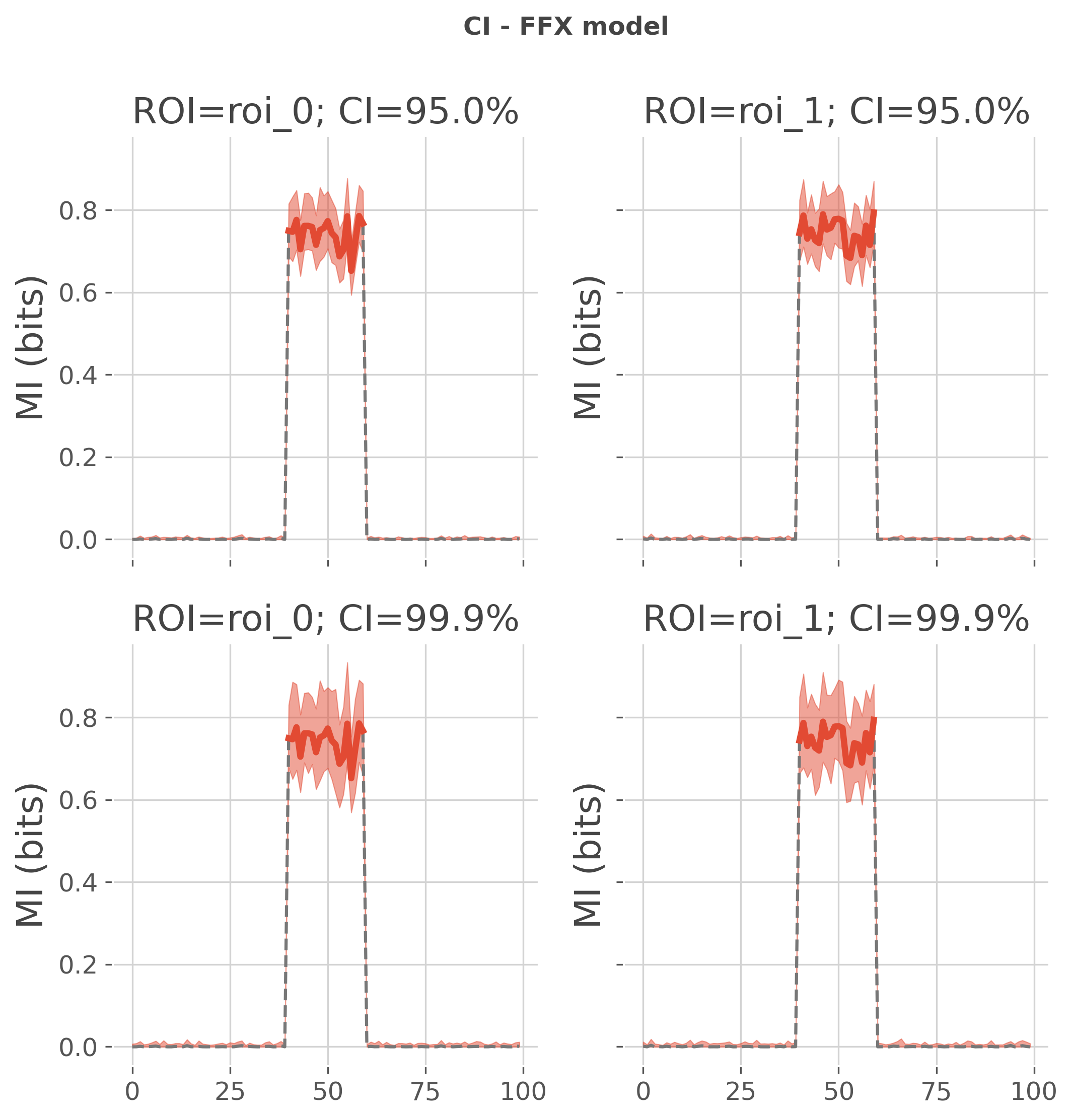
Empirical confidence interval with FFX models#
Then, we estimate the confidence interval when using a fixed-effect model
# computes mi
wf = WfMi(mi_type='cc', inference='ffx')
mi, pv = wf.fit(dt, n_perm=200, n_jobs=1, random_state=0)

# computes confidence interval
ci = wf.confidence_interval(dt, n_boots=200, ci=[95, 99.9], n_jobs=1,
                            random_state=0)
print(ci)

# plot the results
# sphinx_gallery_thumbnail_number = 1
plot(mi, pv, ci, title='CI - FFX model')
plt.show()
  0%|          | Estimating MI : 0/2 [00:00<?,       ?it/s]
 50%|█████     | Estimating MI : 1/2 [00:00<00:00,    4.77it/s]
100%|██████████| Estimating MI : 2/2 [00:00<00:00,    4.94it/s]
100%|██████████| Estimating MI : 2/2 [00:00<00:00,    4.93it/s]

  0%|          | Estimating CI : 0/2 [00:00<?,       ?it/s]
 50%|█████     | Estimating CI : 1/2 [00:00<00:00,    3.87it/s]
100%|██████████| Estimating CI : 2/2 [00:00<00:00,    3.85it/s]
100%|██████████| Estimating CI : 2/2 [00:00<00:00,    3.85it/s]
<xarray.DataArray (ci: 2, bound: 2, times: 100, roi: 2)>
array([[[[-7.23073406e-04, -7.16491298e-04],
         [-7.22913892e-04, -7.21564212e-04],
         [-7.12451612e-04, -3.77852905e-04],
         [-7.21695001e-04, -7.23084135e-04],
         [-7.20416509e-04, -7.22600946e-04],
         [-7.20839755e-04, -7.19997847e-04],
         [-7.21475668e-04, -7.16736185e-04],
         [-7.21381190e-04, -7.22534403e-04],
         [-7.20533649e-04, -7.21103013e-04],
         [-7.21385662e-04, -7.19823394e-04],
         [-7.23042384e-04, -7.21751861e-04],
         [-7.21119570e-04, -7.21950000e-04],
         [-7.17653520e-04, -5.43816230e-04],
         [-7.22834983e-04, -7.22015522e-04],
         [-6.43601312e-04, -7.22082109e-04],
         [-7.20890473e-04, -7.01435236e-04],
         [-7.21521075e-04, -7.06132196e-04],
         [-7.20710467e-04, -7.21843597e-04],
         [-7.22542193e-04, -7.21560745e-04],
         [-7.22901901e-04, -7.22991019e-04],
...
         [ 4.94244866e-03,  1.07339411e-02],
         [ 9.79310366e-03,  4.22542676e-03],
         [ 6.94442050e-03,  8.52263006e-03],
         [ 8.93999326e-03,  1.42579034e-02],
         [ 6.89398717e-03,  1.20471159e-02],
         [ 1.16844222e-02,  4.71777218e-03],
         [ 6.02946251e-03,  5.92530687e-03],
         [ 9.03900810e-03,  4.65719321e-03],
         [ 1.27212104e-02,  6.39466274e-03],
         [ 1.15400850e-02,  1.47285943e-02],
         [ 6.34947684e-03,  4.47972739e-03],
         [ 4.56949591e-03,  4.61853010e-03],
         [ 6.94840438e-03,  4.63257400e-03],
         [ 1.17303262e-02,  9.08010769e-03],
         [ 4.93415462e-03,  1.25797414e-02],
         [ 9.11222803e-03,  6.01635745e-03],
         [ 6.81227519e-03,  1.18603074e-02],
         [ 5.50806255e-03,  1.50310924e-02],
         [ 9.75895521e-03,  1.13908156e-02],
         [ 1.10290457e-02,  7.38632124e-03]]]])
Coordinates:
  * ci       (ci) float64 95.0 99.9
  * bound    (bound) <U4 'low' 'high'
  * times    (times) int64 0 1 2 3 4 5 6 7 8 9 ... 90 91 92 93 94 95 96 97 98 99
  * roi      (roi) <U5 'roi_0' 'roi_1'
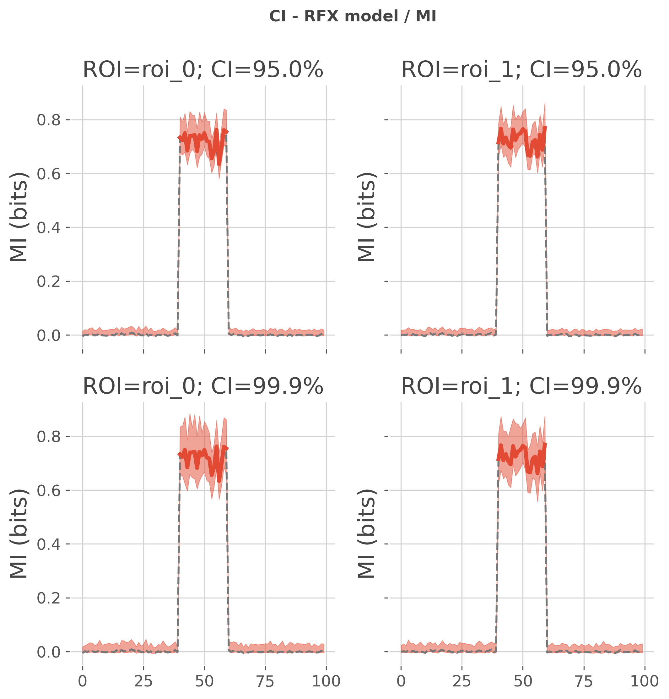
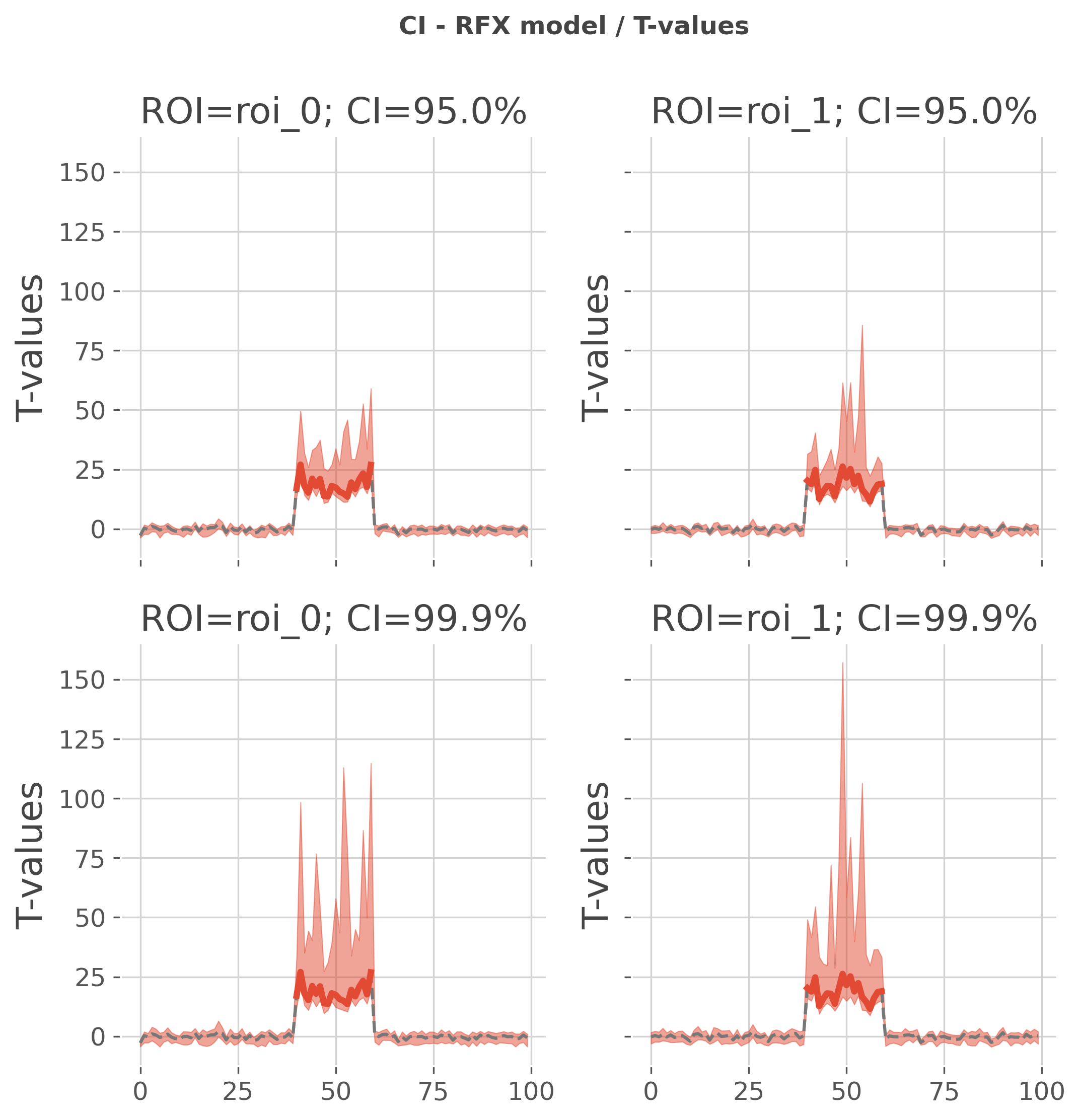
Empirical confidence interval with RFX models#
When using the random-effect model, it’s either possible to estimate the confidence interval on the returned mutual-information or on t-values. To do the switch, you can use the parameter rfx_es for choosing between ‘mi’ or ‘tvalues’
  0%|          | Estimating MI : 0/2 [00:00<?,       ?it/s]
 50%|█████     | Estimating MI : 1/2 [00:01<00:01,    1.08s/it]
100%|██████████| Estimating MI : 2/2 [00:02<00:00,    1.07s/it]
100%|██████████| Estimating MI : 2/2 [00:02<00:00,    1.07s/it]

  0%|          | Estimating CI : 0/2 [00:00<?,       ?it/s]
 50%|█████     | Estimating CI : 1/2 [00:01<00:01,    1.60s/it]
100%|██████████| Estimating CI : 2/2 [00:03<00:00,    1.60s/it]
100%|██████████| Estimating CI : 2/2 [00:03<00:00,    1.60s/it]
confidence interval on t-values
wf = WfMi(mi_type='cc', inference='rfx')
_, pv = wf.fit(dt, n_perm=200, n_jobs=1, random_state=0)
tv = wf.tvalues
ci = wf.confidence_interval(dt, n_boots=200, ci=[95, 99.9], n_jobs=1,
                            random_state=0, rfx_es='tvalues')
plot(tv, pv, ci, title='CI - RFX model / T-values', units='T-values')
plt.show()
  0%|          | Estimating MI : 0/2 [00:00<?,       ?it/s]
 50%|█████     | Estimating MI : 1/2 [00:01<00:01,    1.07s/it]
100%|██████████| Estimating MI : 2/2 [00:02<00:00,    1.07s/it]
100%|██████████| Estimating MI : 2/2 [00:02<00:00,    1.07s/it]

  0%|          | Estimating CI : 0/200 [00:00<?,       ?it/s]
 18%|█▊        | Estimating CI : 36/200 [00:00<00:00, 2239.55it/s]
 36%|███▋      | Estimating CI : 73/200 [00:00<00:00, 2248.31it/s]
 55%|█████▌    | Estimating CI : 110/200 [00:00<00:00, 2255.81it/s]
 72%|███████▎  | Estimating CI : 145/200 [00:00<00:00, 2228.90it/s]
 90%|█████████ | Estimating CI : 181/200 [00:00<00:00, 2230.75it/s]
100%|██████████| Estimating CI : 200/200 [00:00<00:00, 2130.04it/s]
Total running time of the script: (0 minutes 12.203 seconds)
Estimated memory usage: 469 MB