Lag estimation between delayed times-series using the cross-correlation

This example illustrates how to estimate the lags between delayed times-series using the cross-correlation function.

import numpy as np
import xarray as xr

from frites.conn import conn_ccf
from frites import set_mpl_style

import matplotlib.pyplot as plt
set_mpl_style()

Data simulation

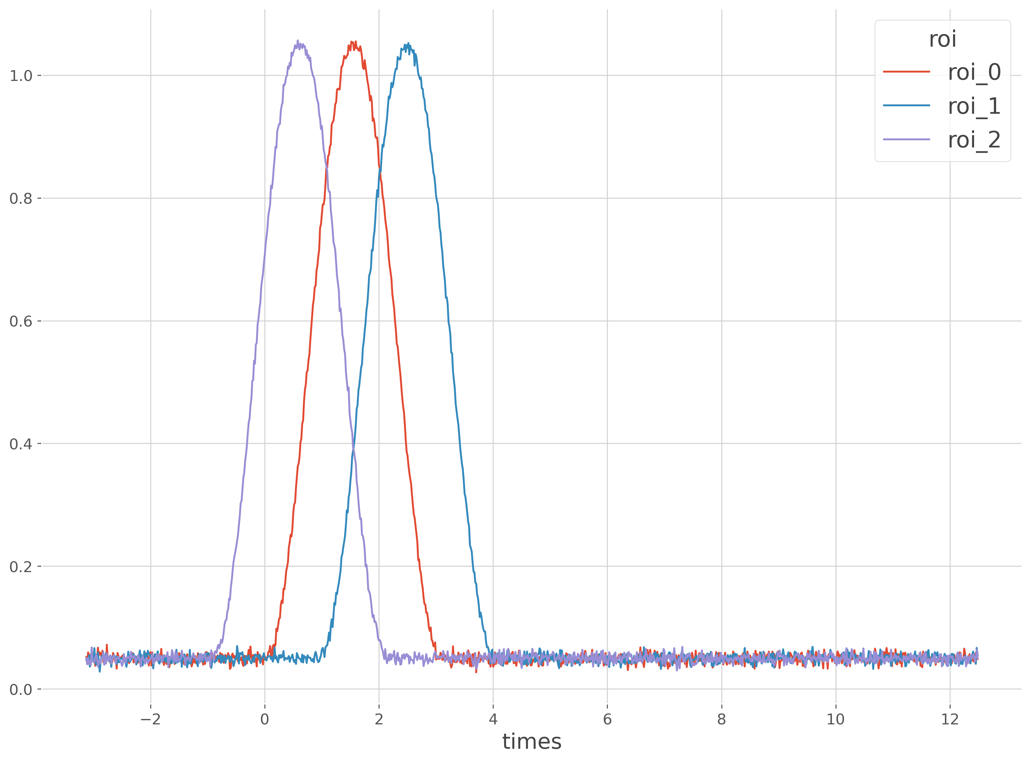
First, let’s start by simulating data and time-series with fixed delays between them.

# number of trials, brain regions and time points
n_trials, n_roi, n_times = 20, 3, 1000

# create coordinates
trials = np.arange(n_trials)
roi = [f"roi_{k}" for k in range(n_roi)]
times = (np.arange(n_times) - 200) / 64.

# data creation
rnd = np.random.RandomState(0)
x = .1 * rnd.rand(n_trials, n_roi, n_times)

"""
lag definition

Here, we use a dict where the keys refer to the target brain region and the
values for the lag value between this target and the first brain region
(considered as a reference here). Positive delays are moving the target from
the source while negative lags are moving the target toward the source.
"""
lags = {
    1: 60,   #  60 samples are separating roi_0 and roi_1
    2: -60,  # -60 samples are separating roi_0 and roi_2
}
bump_len = 200
bump = np.hanning(bump_len).reshape(1, -1)
ref = 200
x[:, 0, ref:ref + bump_len] += bump
for t, lag in lags.items():
    x[:, t, ref + lag:ref + lag + bump_len] += bump

# xarray conversion
x = xr.DataArray(x, dims=('trials', 'roi', 'times'),
                 coords=(trials, roi, times))

# data plotting
x.mean('trials').plot(x='times', hue='roi')
plt.show()

Compute the cross-correlation

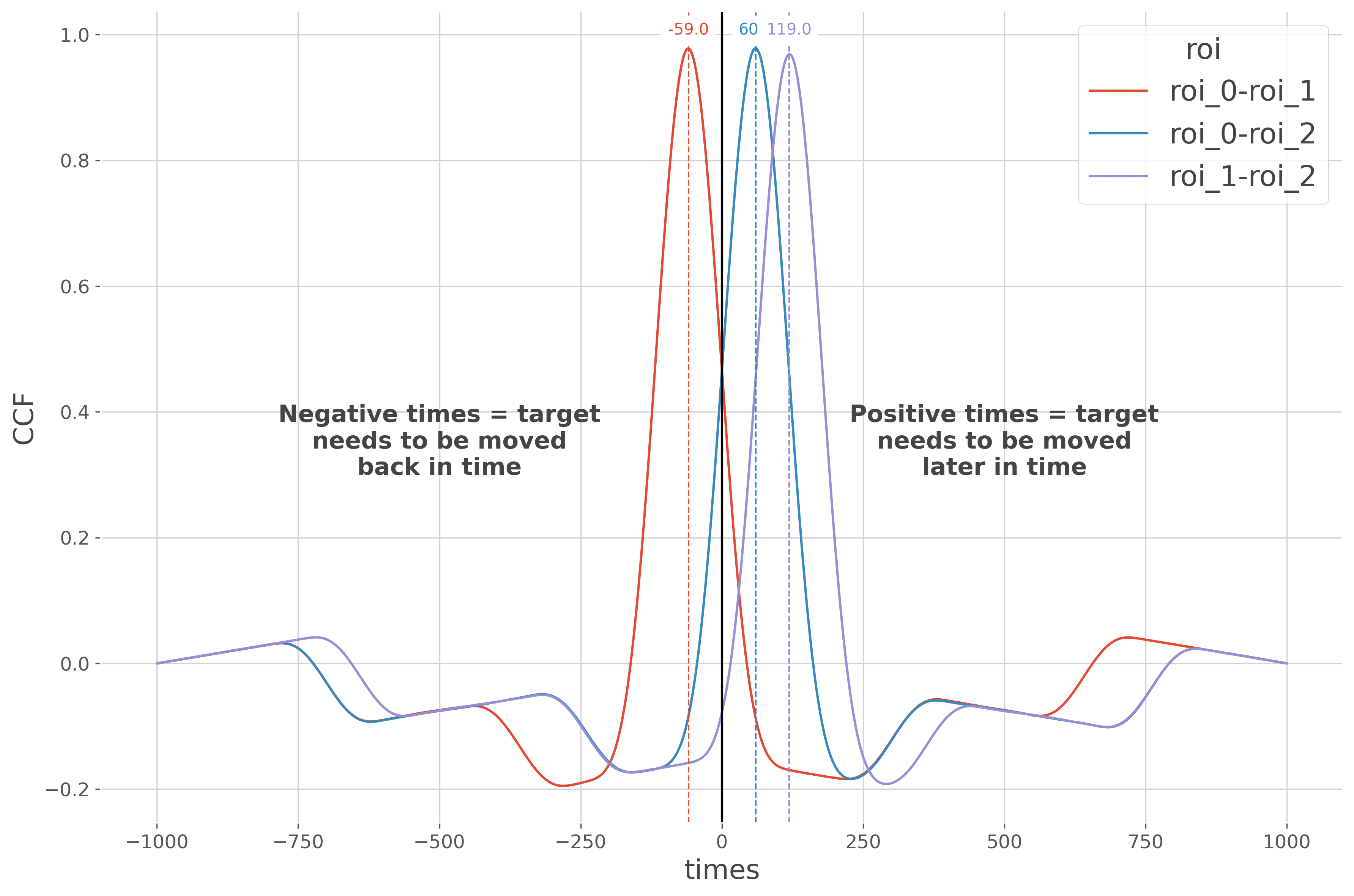
Then, we can try to estimate the delays between the time series using the cross-correlation function

# compute delayed dfc
ccf = conn_ccf(x, times='times', roi='roi', n_jobs=1)

# get lag at maximum peak
ccf_m = ccf.mean('trials')
lags = ccf['times'].data[np.where(ccf_m == ccf_m.max('times'))[1]]

  0%|          | Estimating CCF : 0/3 [00:00<?,       ?it/s]
100%|██████████| Estimating CCF : 3/3 [00:00<00:00,  224.45it/s]

Plot the cross-correlation

In this final part, we plot the cross-correlation between brain regions

# plot the cross correlation
# sphinx_gallery_thumbnail_number = 2
plt.figure(figsize=(12, 8))
plt.title('Delays between brain regions')
ccf_m.plot(x='times', hue='roi')
plt.axvline(0., color='k')

# plot peak informations
for n_p in range(len(lags)):
    plt.axvline(lags[n_p], color=f"C{n_p}", linestyle='--', lw=1)
    t = plt.text(lags[n_p], 1., str(lags[n_p]), color=f"C{n_p}", ha='center')
    t.set_bbox(dict(facecolor='w', edgecolor='w'))

# add text
neg = ("Negative times = target\nneeds to be moved\nback in time")
pos = ("Positive times = target\nneeds to be moved\nlater in time")
plt.text(-500, .3, neg, ha='center', fontsize=15, fontweight='bold')
plt.text(500, .3, pos, ha='center', fontsize=15, fontweight='bold')
plt.tight_layout()

plt.show()

Estimated memory usage: 9 MB