Note
Go to the end to download the full example code.
Estimate the Dynamic Functional Connectivity#
This tutorial illustrates how to compute the Dynamic Functional Connectivity (DFC). In particular, we will adress :
How to estimate the DFC at the single trial-level inside a unique time window
How to estimate the DFC on sliding windows
How to use different estimators (mutual-information, correlation and distance correlation)
What are the strengths and weaknesses of each estimator
import numpy as np
import xarray as xr

from frites.estimator import (GCMIEstimator, CorrEstimator, DcorrEstimator)
from frites.conn import conn_dfc, define_windows
from frites import set_mpl_style

import matplotlib.pyplot as plt
set_mpl_style()

# for reproducibility
np.random.seed(0)
Data simulation#
In this first section, we generate simulated data. We first use random data coming from several brain regions and then we introduce some correlations between the first two brain regions.
n_trials = 100
n_roi = 3
n_times = 250
trials = np.arange(n_trials)
roi = [f"r{n_r}" for n_r in range(n_roi)]
times = np.arange(n_times) / 64.
x = np.random.uniform(-1, 1, (n_trials, n_roi, n_times))

# positive correlation between samples [40, 60]
x[:, 0, 40:60] += .4 * x[:, 1, 40:60]
# negative correlation between samples [90, 110]
x[:, 0, 90:110] -= .4 * x[:, 1, 90:110]
# non-linear but monotone relationship between samples [140, 160]
x[:, 0, 140:160] += .4 * x[:, 1, 140:160] ** 3
# non-linear and non-monotone relationship between samples [190, 210]
x[:, 0, 190:210] += x[:, 1, 190:210] ** 2
Note
To summarize :
Electrophysiological data is a 3D array of shape (100 trials, 3 brain regions, 250 time points)
Brain regions 0 and 1 are positively correlated between samples [40, 60]
Brain regions 0 and 1 are negatively correlated between samples [90, 110]
Brain regions 0 and 1 are positively correlated between samples [140, 160] with a monotone but non-linear relationship
Brain regions 0 and 1 are positively correlated between samples [190, 210] with a non-monotone and non-linear relationship
# dataarray transformation
x = xr.DataArray(x, dims=('trials', 'space', 'times'),
                 coords=(trials, roi, times))
print(x)
<xarray.DataArray (trials: 100, space: 3, times: 250)>
array([[[ 0.09762701,  0.43037873,  0.20552675, ..., -0.63344033,
         -0.71030448, -0.02388744],
        [-0.28877452,  0.88086389,  0.53065051, ..., -0.19657293,
         -0.50317307,  0.01173277],
        [-0.37923835, -0.25393027,  0.04994088, ...,  0.43924032,
          0.93277994,  0.01527109]],

       [[-0.39919263,  0.09900115,  0.86163743, ...,  0.87682404,
         -0.5427069 ,  0.35428229],
        [ 0.18576054, -0.97987261, -0.04834761, ...,  0.02416143,
          0.94352615, -0.27231045],
        [ 0.5758315 ,  0.11058821, -0.20873266, ..., -0.77550001,
         -0.91527191, -0.54451801]],

       [[-0.10641336,  0.67398073, -0.55635194, ..., -0.98188   ,
         -0.61655178, -0.45904532],
        [ 0.23236598, -0.23145365,  0.40681406, ..., -0.03978439,
          0.28772807,  0.00354626],
        [ 0.62303694, -0.04783203,  0.04631198, ...,  0.93401105,
         -0.22486565,  0.37338006]],
...
       [[ 0.53539691, -0.54437834, -0.12765829, ..., -0.32439466,
          0.01350653,  0.60155132],
        [ 0.4122914 , -0.38156304,  0.32681442, ...,  0.65563813,
          0.31738948,  0.92699652],
        [ 0.35586539, -0.7822369 ,  0.13831242, ..., -0.15490871,
          0.41263446,  0.79900583]],

       [[ 0.77639847, -0.49191505,  0.97295482, ..., -0.18097604,
         -0.34969498,  0.84411979],
        [ 0.23698913, -0.52063671,  0.5570413 , ..., -0.93697483,
          0.12883945, -0.17336007],
        [-0.77450055,  0.20179537,  0.67936801, ..., -0.97704647,
         -0.12786805,  0.85446235]],

       [[ 0.46992167,  0.23258818,  0.753783  , ..., -0.11128889,
         -0.17270254,  0.67276573],
        [-0.15935157, -0.36457215, -0.50209665, ..., -0.00973454,
         -0.20538497, -0.25809991],
        [ 0.46541107, -0.22049018, -0.67211057, ...,  0.42287756,
         -0.13557333, -0.61181913]]])
Coordinates:
  * trials   (trials) int64 0 1 2 3 4 5 6 7 8 9 ... 91 92 93 94 95 96 97 98 99
  * space    (space) <U2 'r0' 'r1' 'r2'
  * times    (times) float64 0.0 0.01562 0.03125 0.04688 ... 3.859 3.875 3.891
Computes the DFC in a single temporal window#
In the section we compute the DFC inside a single time-window. Actually, the DFC is going to be computed across the entire time-series
# compute the dfc
dfc = conn_dfc(x, times='times', roi='space')

print(dfc)
  0%|          | Estimating DFC : 0/3 [00:00<?,       ?it/s]
100%|██████████| Estimating DFC : 3/3 [00:00<00:00, 1475.48it/s]
<xarray.DataArray 'DFC (Gaussian Copula Mutual Information Estimator)' (
                                                                        trials: 100,
                                                                        roi: 3,
                                                                        times: 1)>
array([[[1.50026195e-02],
        [6.53586991e-04],
        [3.04782181e-03]],

       [[2.55722110e-03],
        [9.47777648e-04],
        [9.54755058e-04]],

       [[1.91575743e-03],
        [1.65526383e-03],
        [3.67320934e-03]],

       [[9.54645657e-05],
        [1.47084296e-02],
        [1.35143287e-03]],

       [[5.49641764e-03],
        [3.71751172e-04],
        [2.98313168e-03]],

...

       [[7.03146361e-05],
        [9.66168381e-03],
        [1.17242755e-03]],

       [[1.41984574e-03],
        [2.23128637e-03],
        [5.71009004e-03]],

       [[1.88476965e-03],
        [3.06461961e-03],
        [7.38627603e-03]],

       [[1.62730534e-02],
        [3.54107120e-03],
        [3.26337272e-06]],

       [[4.45268088e-05],
        [1.45566883e-03],
        [3.73451796e-04]]])
Coordinates:
  * trials   (trials) int64 0 1 2 3 4 5 6 7 8 9 ... 91 92 93 94 95 96 97 98 99
  * roi      (roi) <U5 'r0-r1' 'r0-r2' 'r1-r2'
  * times    (times) float64 1.945
Attributes:
    win_sample:  [  0 249]
    win_times:   [1.9453125]
    agg_ch:      0
    type:        dfc
    estimator:   Gaussian Copula Mutual Information Estimator
    unit:        Bits
    sfreq:       64.0
    sources:     [0, 0, 1]
    targets:     [1, 2, 2]
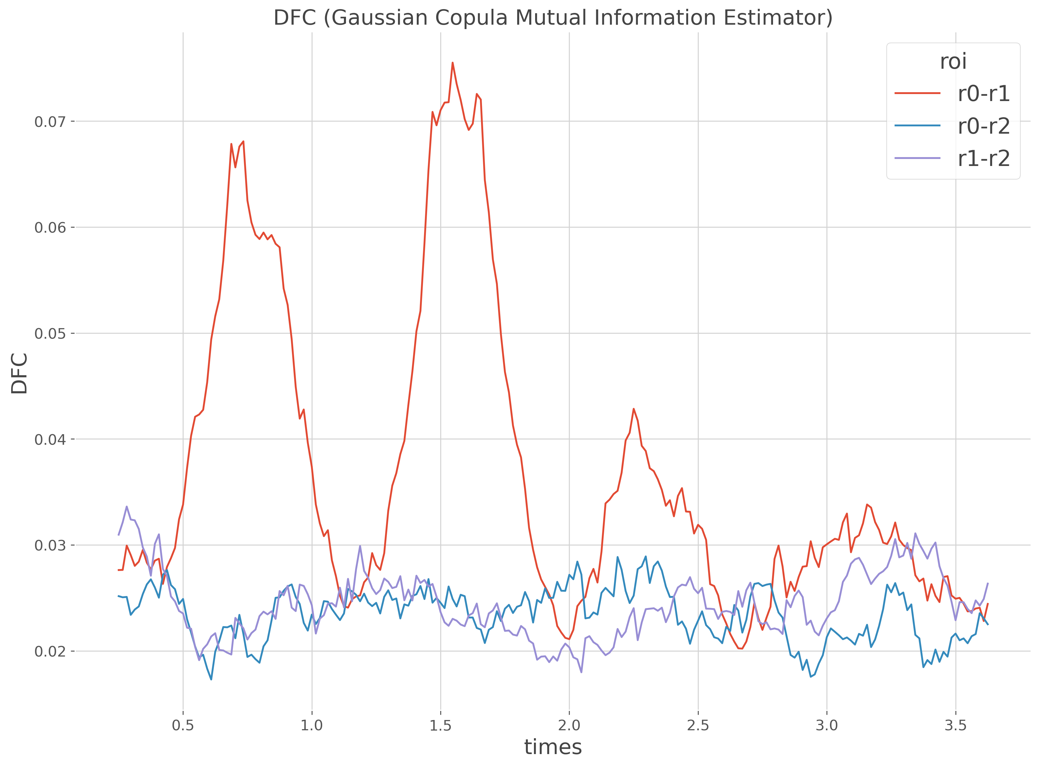
Computes the DFC on sliding windows#
In this section, we are going to define sliding windows and then compute the DFC inside each one of them.
slwin_len = .5    # windows of length 500ms
slwin_step = .02  # 20ms step between each window (or 480ms overlap)

# define the sliding windows
sl_win = define_windows(times, slwin_len=slwin_len, slwin_step=slwin_step)[0]
print(sl_win)

# compute the DFC on sliding windows
dfc = conn_dfc(x, times='times', roi='space', win_sample=sl_win)

# takes the mean over trials
dfc_m = dfc.mean('trials').squeeze()

# plot the mean over trials
dfc_m.plot.line(x='times', hue='roi')
plt.title(dfc.name), plt.ylabel('DFC')
plt.show()
[[  0  32]
 [  1  33]
 [  2  34]
 [  3  35]
 [  4  36]
 [  5  37]
 [  6  38]
 [  7  39]
 [  8  40]
 [  9  41]
 [ 10  42]
 [ 11  43]
 [ 12  44]
 [ 13  45]
 [ 14  46]
 [ 15  47]
 [ 16  48]
 [ 17  49]
 [ 18  50]
 [ 19  51]
 [ 20  52]
 [ 21  53]
 [ 22  54]
 [ 23  55]
 [ 24  56]
 [ 25  57]
 [ 26  58]
 [ 27  59]
 [ 28  60]
 [ 29  61]
 [ 30  62]
 [ 31  63]
 [ 32  64]
 [ 33  65]
 [ 34  66]
 [ 35  67]
 [ 36  68]
 [ 37  69]
 [ 38  70]
 [ 39  71]
 [ 40  72]
 [ 41  73]
 [ 42  74]
 [ 43  75]
 [ 44  76]
 [ 45  77]
 [ 46  78]
 [ 47  79]
 [ 48  80]
 [ 49  81]
 [ 50  82]
 [ 51  83]
 [ 52  84]
 [ 53  85]
 [ 54  86]
 [ 55  87]
 [ 56  88]
 [ 57  89]
 [ 58  90]
 [ 59  91]
 [ 60  92]
 [ 61  93]
 [ 62  94]
 [ 63  95]
 [ 64  96]
 [ 65  97]
 [ 66  98]
 [ 67  99]
 [ 68 100]
 [ 69 101]
 [ 70 102]
 [ 71 103]
 [ 72 104]
 [ 73 105]
 [ 74 106]
 [ 75 107]
 [ 76 108]
 [ 77 109]
 [ 78 110]
 [ 79 111]
 [ 80 112]
 [ 81 113]
 [ 82 114]
 [ 83 115]
 [ 84 116]
 [ 85 117]
 [ 86 118]
 [ 87 119]
 [ 88 120]
 [ 89 121]
 [ 90 122]
 [ 91 123]
 [ 92 124]
 [ 93 125]
 [ 94 126]
 [ 95 127]
 [ 96 128]
 [ 97 129]
 [ 98 130]
 [ 99 131]
 [100 132]
 [101 133]
 [102 134]
 [103 135]
 [104 136]
 [105 137]
 [106 138]
 [107 139]
 [108 140]
 [109 141]
 [110 142]
 [111 143]
 [112 144]
 [113 145]
 [114 146]
 [115 147]
 [116 148]
 [117 149]
 [118 150]
 [119 151]
 [120 152]
 [121 153]
 [122 154]
 [123 155]
 [124 156]
 [125 157]
 [126 158]
 [127 159]
 [128 160]
 [129 161]
 [130 162]
 [131 163]
 [132 164]
 [133 165]
 [134 166]
 [135 167]
 [136 168]
 [137 169]
 [138 170]
 [139 171]
 [140 172]
 [141 173]
 [142 174]
 [143 175]
 [144 176]
 [145 177]
 [146 178]
 [147 179]
 [148 180]
 [149 181]
 [150 182]
 [151 183]
 [152 184]
 [153 185]
 [154 186]
 [155 187]
 [156 188]
 [157 189]
 [158 190]
 [159 191]
 [160 192]
 [161 193]
 [162 194]
 [163 195]
 [164 196]
 [165 197]
 [166 198]
 [167 199]
 [168 200]
 [169 201]
 [170 202]
 [171 203]
 [172 204]
 [173 205]
 [174 206]
 [175 207]
 [176 208]
 [177 209]
 [178 210]
 [179 211]
 [180 212]
 [181 213]
 [182 214]
 [183 215]
 [184 216]
 [185 217]
 [186 218]
 [187 219]
 [188 220]
 [189 221]
 [190 222]
 [191 223]
 [192 224]
 [193 225]
 [194 226]
 [195 227]
 [196 228]
 [197 229]
 [198 230]
 [199 231]
 [200 232]
 [201 233]
 [202 234]
 [203 235]
 [204 236]
 [205 237]
 [206 238]
 [207 239]
 [208 240]
 [209 241]
 [210 242]
 [211 243]
 [212 244]
 [213 245]
 [214 246]
 [215 247]
 [216 248]]

  0%|          | Estimating DFC : 0/3 [00:00<?,       ?it/s]
 33%|███▎      | Estimating DFC : 1/3 [00:00<00:00,   32.52it/s]
 67%|██████▋   | Estimating DFC : 2/3 [00:00<00:00,   33.08it/s]
100%|██████████| Estimating DFC : 3/3 [00:00<00:00,   33.39it/s]
100%|██████████| Estimating DFC : 3/3 [00:00<00:00,   33.24it/s]
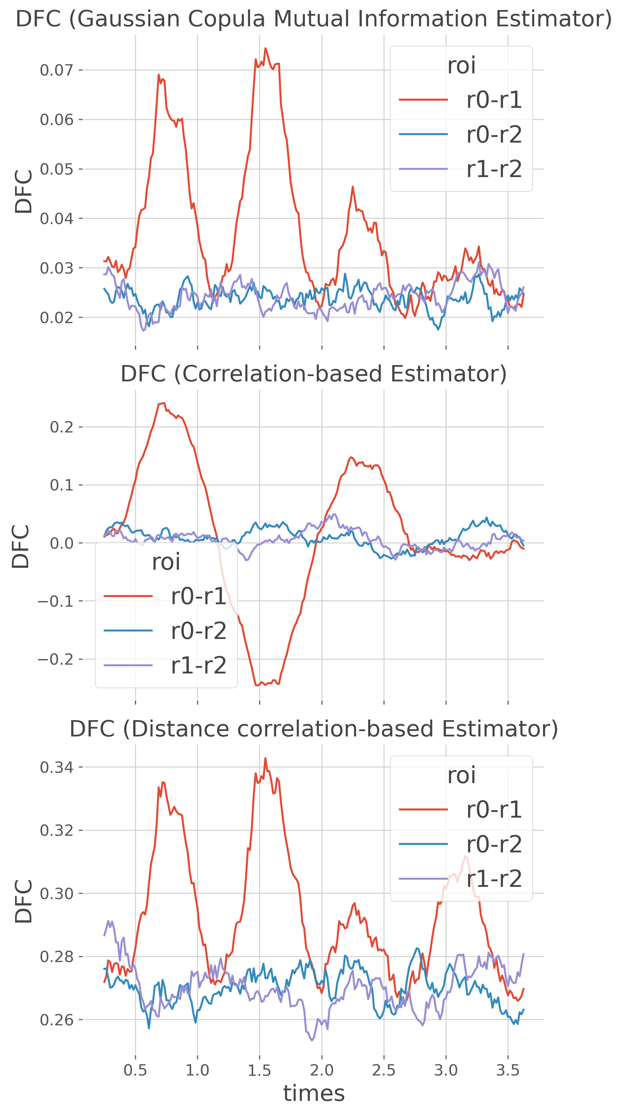
Comparison of several estimators#
By default, the conn_dfc function uses the Gaussian-Copula Mutual-Information (GCMI) estimator. However, the conn_dfc function allows to provide other estimators as soon as it is made for computing information between two continuous variables (mi_type=’cc’). In this final section, we are going to use different estimators, especially the standard correlation and the distance correlation.
est_mi = GCMIEstimator('cc', copnorm=None, biascorrect=False)
est_corr = CorrEstimator()
est_dcorr = DcorrEstimator()

fig, axs = plt.subplots(nrows=3, ncols=1, sharex=True, figsize=(6, 12))

for n_e, est in enumerate([est_mi, est_corr, est_dcorr]):
    # compute the dfc
    dfc = conn_dfc(x, times='times', roi='space', win_sample=sl_win,
                   estimator=est)

    # take the mean across trials
    dfc_m = dfc.mean('trials')

    # plot the result
    plt.sca(axs[n_e])
    dfc_m.plot.line(x='times', hue='roi', ax=plt.gca())
    plt.title(dfc.name)
    plt.ylabel('DFC')
    if n_e != 2: plt.xlabel('')

plt.tight_layout()
plt.show()
  0%|          | Estimating DFC : 0/3 [00:00<?,       ?it/s]
 33%|███▎      | Estimating DFC : 1/3 [00:00<00:01,    1.91it/s]
 67%|██████▋   | Estimating DFC : 2/3 [00:01<00:00,    1.92it/s]
100%|██████████| Estimating DFC : 3/3 [00:01<00:00,    1.92it/s]
100%|██████████| Estimating DFC : 3/3 [00:01<00:00,    1.92it/s]

  0%|          | Estimating DFC : 0/3 [00:00<?,       ?it/s]
 33%|███▎      | Estimating DFC : 1/3 [00:01<00:03,    1.56s/it]
 67%|██████▋   | Estimating DFC : 2/3 [00:03<00:01,    1.56s/it]
100%|██████████| Estimating DFC : 3/3 [00:04<00:00,    1.55s/it]
100%|██████████| Estimating DFC : 3/3 [00:04<00:00,    1.55s/it]

  0%|          | Estimating DFC : 0/3 [00:00<?,       ?it/s]
 33%|███▎      | Estimating DFC : 1/3 [00:01<00:02,    1.14s/it]
 67%|██████▋   | Estimating DFC : 2/3 [00:02<00:01,    1.14s/it]
100%|██████████| Estimating DFC : 3/3 [00:03<00:00,    1.14s/it]
100%|██████████| Estimating DFC : 3/3 [00:03<00:00,    1.14s/it]
Note
To summarize :
GCMI estimators offers a great sensibility. However, the mutual-information is unsigned and therefore, negative correlations are captured as positive information (cf. second bump). In addition, non-monotone relations are not well captured
On the other hand, the correlation clearly extract both positive and negative correlations however, non-monotone relationships are missed. Finally, the correlation is probably not as sensible as the GCMI
Finally, the distance correlation captures all relations but as the GCMI, it is an unsigned measure, missing negative correlations. It is the most powerful estimator however, it is also slower to compute.
Total running time of the script: (1 minutes 46.932 seconds)
Estimated memory usage: 825 MB