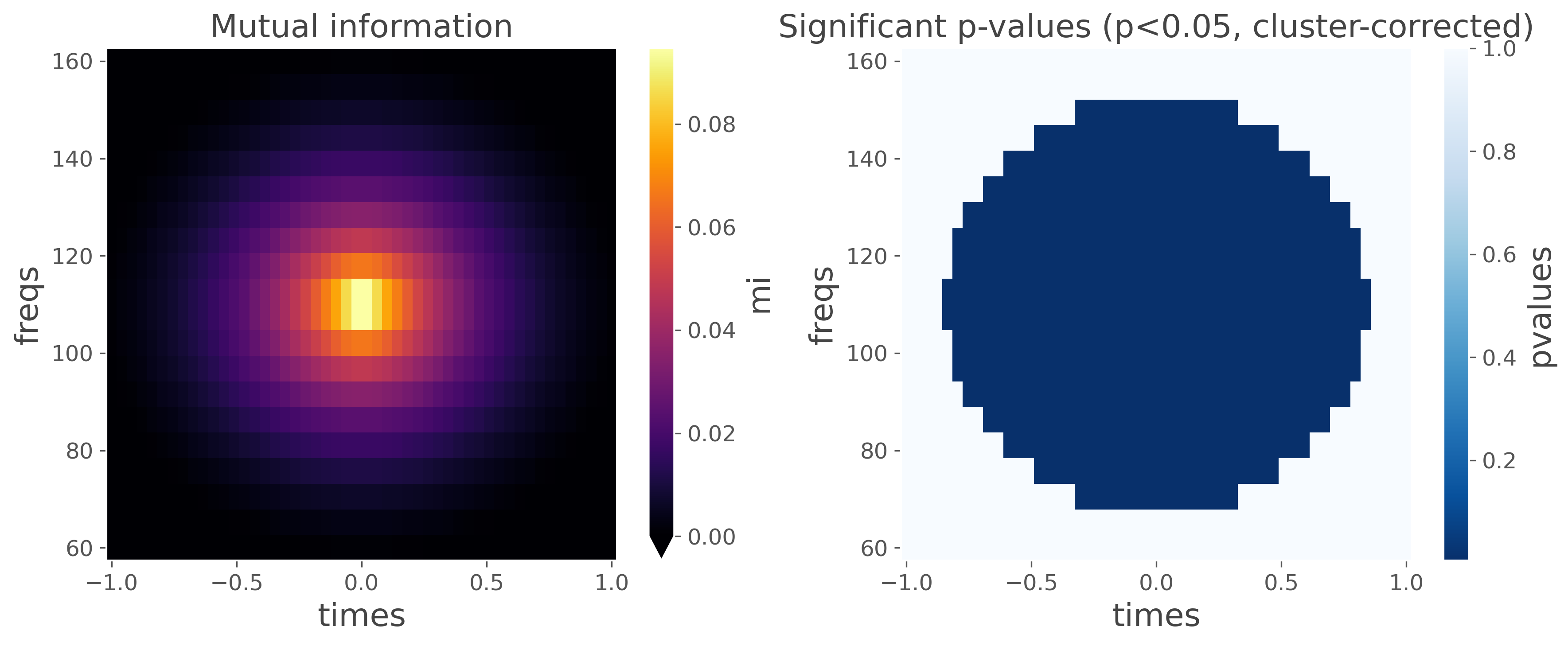
Compute MI across time and frequencies

This example illustrates how to compute the mutual information with time-frequency inputs (e.g time-frequency maps). Then, it uses cluster-based to correct for multiple comparisons.

import numpy as np
import xarray as xr

from frites.dataset import DatasetEphy
from frites.workflow import WfMi
from frites import set_mpl_style

import matplotlib.pyplot as plt
set_mpl_style()

np.random.seed(0)

Simulate data

First, we simulate time-frequency data coming from multiple subjects with a variable number of trials. For a single subject, the data is based on normals (with an addition of noise). The regressor variable is going to be continuous and is also going to be a normal.

# dataset parameters
n_subjects = 5
n_freqs = 20
n_times = 50
n_trials = np.random.randint(50, 100, n_subjects)

function to simulate a single subject

def sim_single_subject(n_freqs, n_times, n_trials, noise_level=10.):
    # generate the mask modulating the amplitude of the gaussian
    t_range, f_range = np.linspace(-1, 1, n_times), np.linspace(-1, 1, n_freqs)
    x, y = np.meshgrid(t_range, f_range)
    d = np.sqrt(x * x + y * y)
    sigma, mu = 2.0, 0.0
    mask_2d = np.exp(-((d - mu) ** .5 / (2. * sigma ** .5)))
    # [0, 1] normalize the mask
    mask_2d -= mask_2d.min()
    mask_2d /= mask_2d.max()
    # turn the mask 3d
    mask_3d = np.tile(mask_2d[np.newaxis, ...], (n_trials, 1, 1))
    # generate the base data
    noise = np.random.uniform(0, noise_level, (n_trials, 1, 1))
    gauss = np.random.normal(0, 1, (n_trials))
    y = gauss.copy()
    gauss = np.tile(gauss.reshape(-1, 1, 1), (1, n_freqs, n_times))
    # data is finally defined as util signal + noise
    data = noise + gauss * mask_3d

    return data[:, np.newaxis, ...], y

simulate multiple subjects and build the dataset container

x, y, roi = [], [], []
times = np.linspace(-1, 1, n_times)
freqs = np.linspace(60, 160, n_freqs)
for s, tr in zip(range(n_subjects), n_trials):
    # simulate the data coming from a single subject
    x_single_suj, y_single_suj = sim_single_subject(n_freqs, n_times, tr)
    # xarray conversion
    _x = xr.DataArray(x_single_suj, dims=('trials', 'roi', 'freqs', 'times'),
                      coords=(y_single_suj, ['roi_0'], freqs, times))
    x += [_x]

# define an instance of DatasetEphy
ds = DatasetEphy(x, y='trials', roi='roi', times='times')

Compute the mutual information

Then we compute the quantity of information shared by the time-frequency data and the continuous regressor

# compute the mutual information
wf = WfMi(inference='ffx', mi_type='cc')
mi, pv = wf.fit(ds, n_perm=200, mcp='cluster', random_state=0, n_jobs=1)

  0%|          | Estimating MI : 0/1 [00:00<?,       ?it/s]
100%|██████████| Estimating MI : 1/1 [00:00<00:00,    1.26it/s]
100%|██████████| Estimating MI : 1/1 [00:00<00:00,    1.26it/s]

plot the mutual information and p-values

plt.figure(figsize=(12, 5))
plt.subplot(1, 2, 1)
mi.squeeze().plot.pcolormesh(vmin=0, cmap='inferno')
plt.title('Mutual information')
plt.subplot(1, 2, 2)
pv.squeeze().plot.pcolormesh(cmap='Blues_r')
plt.title('Significant p-values (p<0.05, cluster-corrected)')
plt.tight_layout()
plt.show()

Estimated memory usage: 9 MB