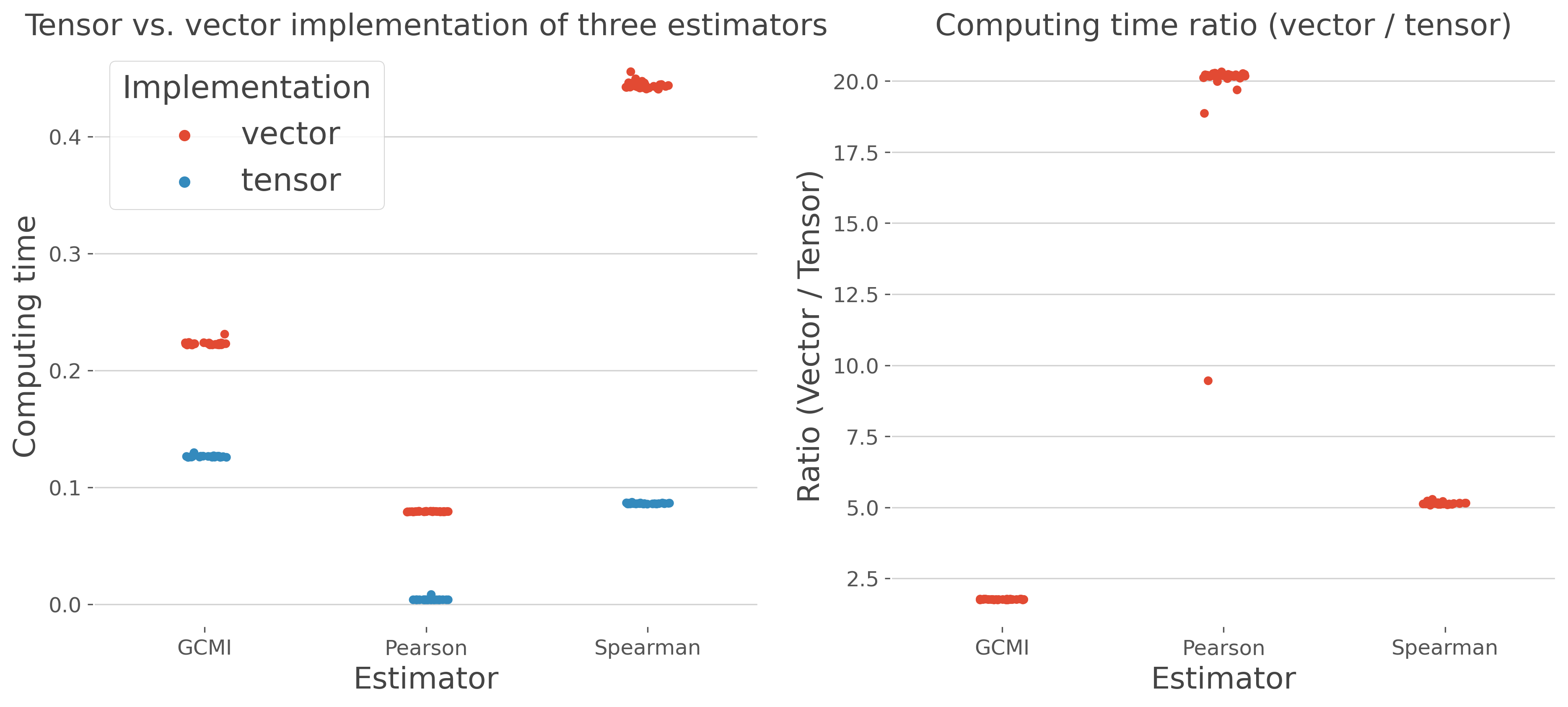
Comparison between tensor and vector based computations

In this example, we compared the elapsed computing time when using a vector based implementation (i.e. operations between vectors inside nested for loops) with a tensor-based implementation (i.e. operations on the full array at once).

import numpy as np
import pandas as pd

from frites.estimator import GCMIEstimator, CorrEstimator
from frites import set_mpl_style

from time import time

import matplotlib.pyplot as plt
import seaborn as sns
set_mpl_style()

Define a dataset

In this first section, we define two multi-dimensional variables x and y

# shape of the two variables
shape = (1000, 1, 400)

# define the x and y variables
x = np.random.rand(*shape)
y = np.random.rand(*shape)

Define vector- and tensor-based estimators

Next, we define three estimators of information : Gaussian-Copula Mutual information, Pearson and Spearman correlations with both vector and tensor-based computations

# vector-based estimators
vec_est = {
    'GCMI': GCMIEstimator(mi_type='cc', tensor=False),
    'Pearson': CorrEstimator(implementation='vector'),
    'Spearman': CorrEstimator(method='spearman', implementation='vector'),
}

# tensor-based estimators
ten_est = {
    'GCMI': GCMIEstimator(mi_type='cc', tensor=True),
    'Pearson': CorrEstimator(implementation='tensor'),
    'Spearman': CorrEstimator(method='spearman', implementation='tensor'),
}

Computing time estimation

In this first section, we define two multi-dimensional variables x and y

# number of loops for repeating computations
n_loops = 30

# function for estimating the computing time

def computing_time(estimator):
    """Estimate computing time."""
    tot_time = []
    for k in range(n_loops):
        start = time()
        estimator.estimate(x, y)
        end = time()
        tot_time.append(end - start)
    return tot_time

# computing time for all of the methods
meth_name, meth_imp, comp_time, comp_name, comp_ratio = [], [], [], [], []
for name in vec_est.keys():
    # vector computations
    meth_name += [name] * n_loops
    meth_imp += ['vector'] * n_loops
    _time_vec = computing_time(vec_est[name])
    comp_time += _time_vec

    # tensor computations
    meth_name += [name] * n_loops
    meth_imp += ['tensor'] * n_loops
    _time_ten = computing_time(ten_est[name])
    comp_time += _time_ten

    # computing time ratio
    comp_name += [name] * n_loops
    comp_ratio += (np.array(_time_vec) / np.array(_time_ten)).tolist()

# merge the results in a dataframe
results = pd.DataFrame({
   "Estimator": meth_name,
   "Implementation": meth_imp,
   "Computing time": comp_time,
})
results_comp = pd.DataFrame({
   "Estimator": comp_name,
   "Ratio (Vector / Tensor)": comp_ratio
})

# plot the results
plt.figure(figsize=(15, 6))
plt.subplot(121)
sns.stripplot(
    data=results, x='Estimator', y='Computing time', hue='Implementation'
)
plt.title("Tensor vs. vector implementation of three estimators")

plt.subplot(122)
sns.stripplot(
    data=results_comp, x='Estimator', y='Ratio (Vector / Tensor)',
)
plt.title("Computing time ratio (vector / tensor)")
plt.show()

Note

As shown in the results, the tensor-based implementations are at least twice as fast compared to the vector-based computations

Estimated memory usage: 15 MB