MI between a continuous and a discret variables

This example illustrates how to compute the mutual information between a continuous and a discret variables. The first variable is an electrophysiological data (M/EEG, intracranial). The discret variable, composed with integers, can for example describe conditions. This type of mutual information is equivalent to was is performed in machine-learning. For further details, see Ince et al., 2017 [12]

from frites.simulations import sim_multi_suj_ephy, sim_mi_cd
from frites.dataset import DatasetEphy
from frites.workflow import WfMi
from frites import set_mpl_style

import matplotlib.pyplot as plt
set_mpl_style()

Simulate electrophysiological data

Let’s start by simulating MEG / EEG electrophysiological data coming from multiple subjects using the function frites.simulations.sim_multi_suj_ephy(). As a result, the x output is a list of length n_subjects of arrays, each one with a shape of n_epochs, n_sites, n_times

modality = 'meeg'
n_subjects = 5
n_epochs = 400
n_times = 100
x, roi, time = sim_multi_suj_ephy(n_subjects=n_subjects, n_epochs=n_epochs,
                                  n_times=n_times, modality=modality,
                                  random_state=0)

Extract the discret variable

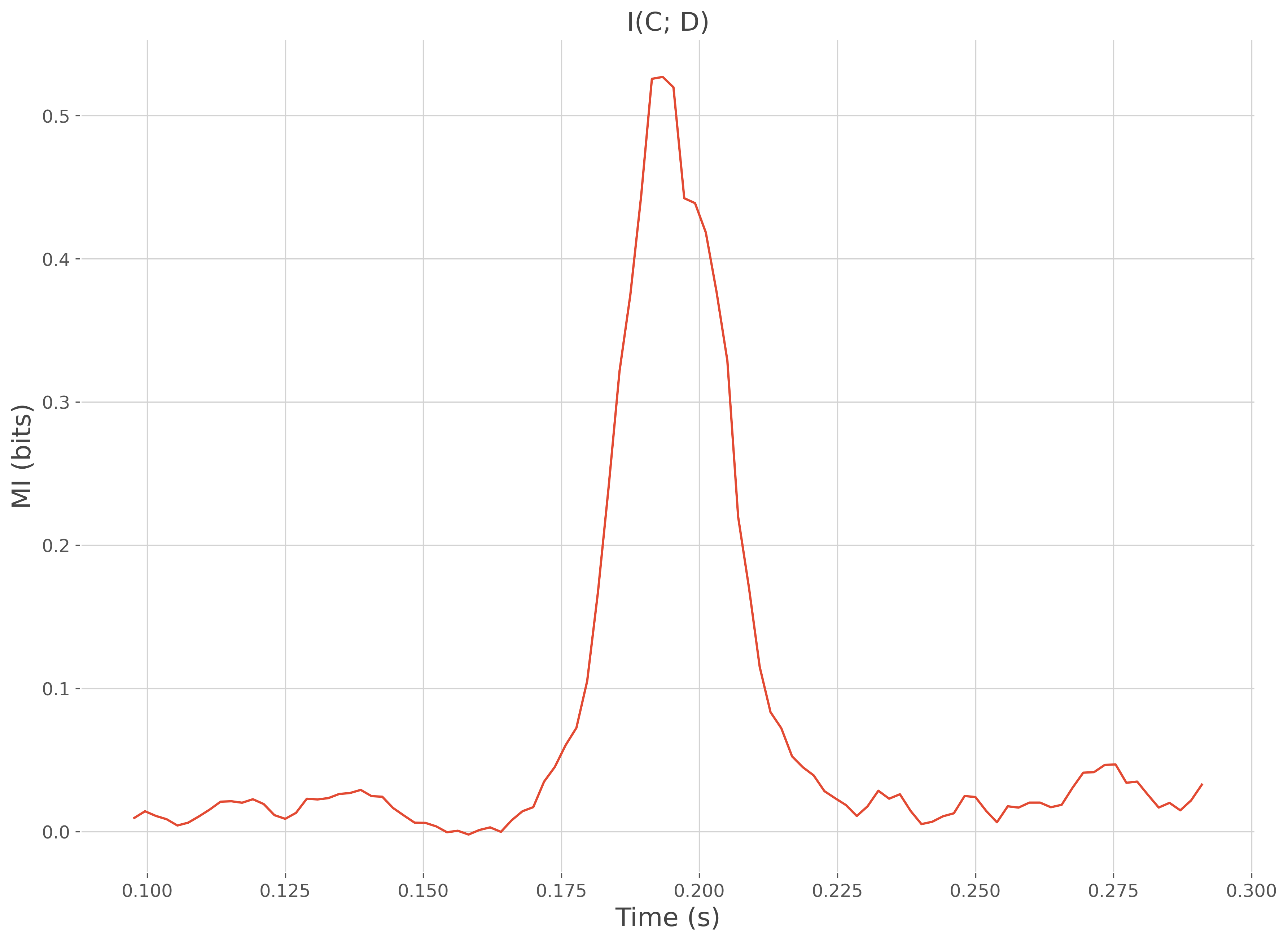
As explains in the top description, the discret variable is used to describes for example conditions. Thus, by computing the mutual information between the electrophysiological data and your discret variable, you are looking for recording sites and time-points of data that correlates with conditions. This kind of analysis is similar to what is done in machine-learning. First, extract the conditions from the random dataset generated above.

x, y, _ = sim_mi_cd(x, snr=1., n_conditions=3)
# print the conditions for the single subject
print(y[0])

[0 0 0 0 0 0 0 0 0 0 0 0 0 0 0 0 0 0 0 0 0 0 0 0 0 0 0 0 0 0 0 0 0 0 0 0 0
 0 0 0 0 0 0 0 0 0 0 0 0 0 0 0 0 0 0 0 0 0 0 0 0 0 0 0 0 0 0 0 0 0 0 0 0 0
 0 0 0 0 0 0 0 0 0 0 0 0 0 0 0 0 0 0 0 0 0 0 0 0 0 0 0 0 0 0 0 0 0 0 0 0 0
 0 0 0 0 0 0 0 0 0 0 0 0 0 0 0 0 0 0 0 0 0 0 0 1 1 1 1 1 1 1 1 1 1 1 1 1 1
 1 1 1 1 1 1 1 1 1 1 1 1 1 1 1 1 1 1 1 1 1 1 1 1 1 1 1 1 1 1 1 1 1 1 1 1 1
 1 1 1 1 1 1 1 1 1 1 1 1 1 1 1 1 1 1 1 1 1 1 1 1 1 1 1 1 1 1 1 1 1 1 1 1 1
 1 1 1 1 1 1 1 1 1 1 1 1 1 1 1 1 1 1 1 1 1 1 1 1 1 1 1 1 1 1 1 1 1 1 1 1 1
 1 1 1 1 1 1 1 1 2 2 2 2 2 2 2 2 2 2 2 2 2 2 2 2 2 2 2 2 2 2 2 2 2 2 2 2 2
 2 2 2 2 2 2 2 2 2 2 2 2 2 2 2 2 2 2 2 2 2 2 2 2 2 2 2 2 2 2 2 2 2 2 2 2 2
 2 2 2 2 2 2 2 2 2 2 2 2 2 2 2 2 2 2 2 2 2 2 2 2 2 2 2 2 2 2 2 2 2 2 2 2 2
 2 2 2 2 2 2 2 2 2 2 2 2 2 2 2 2 2 2 2 2 2 2 2 2 2 2 2 2 2 2]

Define the electrophysiological dataset

Now we define an instance of frites.dataset.DatasetEphy

dt = DatasetEphy(x, y=y, roi=roi, times=time)

Compute the mutual information

Once we have the dataset instance, we can then define an instance of workflow frites.workflow.WfMi. This instance is used to compute the mutual information

# mutual information type ('cd' = continuous / discret)
mi_type = 'cd'

# define the workflow
wf = WfMi(mi_type=mi_type, verbose=False)
# compute the mutual information
mi, _ = wf.fit(dt, mcp=None, n_jobs=1)

# plot the information shared between the data and the regressor y
plt.plot(time, mi)
plt.xlabel("Time (s)"), plt.ylabel("MI (bits)")
plt.title('I(C; D)')
plt.show()

Estimated memory usage: 9 MB