
frites.simulations.StimSpecAR#
- class frites.simulations.StimSpecAR(verbose=None)[source]#
Stimulus-specific autoregressive (AR) Model.
This class can be used to simulate several networks where the information sent between node is stimulus specific inside a temporal region.
- Attributes:
Methods
compute_covgc(ar[, dt, lag, step, method, ...])Compute the Covariance-based Granger Causality.
fit([ar_type, sf, n_times, n_epochs, dt, ...])Get the data generated by the selected model.
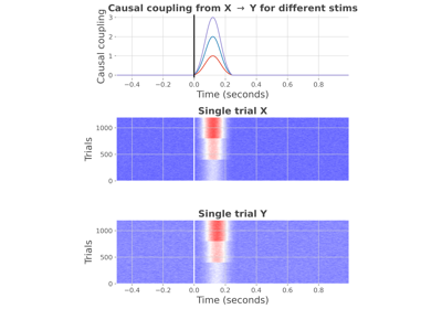
plot([psd, cmap, colorbar])Plot the generated data.
plot_covgc([gc, plot_mi])Plot the Granger Causality.
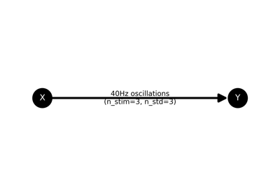
Plot the model of the network.
- property ar#
Output data generated by the selected model.
- compute_covgc(ar, dt=50, lag=5, step=1, method='gc', conditional=False)[source]#
Compute the Covariance-based Granger Causality.
In addition of computing the Granger Causality, the mutual-information between the Granger causalitity and the stimulus is also computed.
- Parameters:
- dt
int Duration of the time window for covariance correlation in samples
- lag
int Number of samples for the lag within each trial
- step
int| 1 Number of samples stepping between each sliding window onset
- method{‘gauss’, ‘gc’}
Method for the estimation of the covgc. Use either ‘gauss’ which assumes that the time-points are normally distributed or ‘gc’ in order to use the gaussian-copula.
- dt
- Returns:
- gcnumpy:array_like
Granger Causality arranged as (n_epochs, n_pairs, n_windows, 3) where the last dimension means :
0 : pairs[:, 0] -> pairs[:, 1] (x->y)
1 : pairs[:, 1] -> pairs[:, 0] (y->x)
2 : instantaneous (x.y)
- fit(ar_type='hga', sf=200, n_times=300, n_epochs=100, dt=50, n_stim=3, n_std=3, stim_onset=100, random_state=None)[source]#
Get the data generated by the selected model.
- Parameters:
- ar_type{‘hga’, ‘osc_20’, ‘osc_40’, ‘ding_2’, ‘ding_3’, ‘ding_5’}
Autoregressive model type. Choose either :
‘hga’ : for evoked high-gamma activity
‘osc_20’ / ‘osc_40’ : for oscillations respectively around 20Hz and 40Hz
‘osc_40_3’ : oscillations at 40hz for 3 nodes. This model simulates X->Y, X->Z and instantaneous Y.Z
‘ding_2’ / ‘ding_3_direct’ / ‘ding_3_indirect’ / ‘ding_5’ : respectively the models with 2, 3 or 5 nodes described by Ding et al. [7]
- sf
float| 200 The sampling frequency
- n_times
int| 300 Number of time points
- n_epochs
int| 100 Number of epochs
- dt
int| 50 Width of the time-varying Gaussian stimulus
- n_stim
int| 3 Number of stimulus to use
- n_std
float,int| 3 Number of standard deviations the stimulus exceed the random noise. Should be an integer striclty over 1. Note that this concerns the first stimulus. For example, if n_std=3, the first stimulus is going to have a deviation 3 times larger than the noise, the second stimulus 6 times the noise, the third stimulus 9 times.
- stim_onset
int| 100 Index where the time-varying Gaussian stimulus should start
- random_state
int|None Fix the random state of the machine for reproducibility
- Returns:
- data
xarray.DataArray DataArray of shape (n_epochs * n_stim, n_roi, n_times)
- data
Examples using
fit: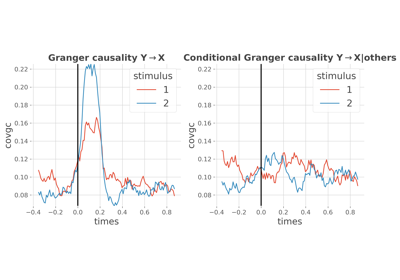
AR : conditional covariance based Granger Causality
AR : conditional covariance based Granger Causality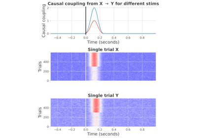
PID: Decomposing the information carried by pairs of brain regions
PID: Decomposing the information carried by pairs of brain regions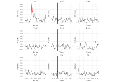
Statistical analysis of a stimulus-specific network
Statistical analysis of a stimulus-specific network
- property gc#
Granger causality.
- property mi#
Mutual-information between the granger causality and stimulus.
- plot(psd=False, cmap='plasma', colorbar=False, **kwargs)[source]#
Plot the generated data.
- Parameters:
Examples using
plot:
PID: Decomposing the information carried by pairs of brain regions
PID: Decomposing the information carried by pairs of brain regions
- plot_covgc(gc=None, plot_mi=False)[source]#
Plot the Granger Causality.
Note that before plotting the Granger causality, the method
StimSpecAR.compute_covgchave to be launched before.- Parameters:
- gc
DataArray|None Granger Causality output of the function
frites.conn.conn_covgc()- plot_mibool |
False If False (default) the Granger causality is plotted. If True, it is the information shared between the Granger causality and the stimulus that is plotted.
- gc
Examples using
plot_covgc:
AR : conditional covariance based Granger Causality
AR : conditional covariance based Granger Causality
- plot_model()[source]#
Plot the model of the network.
Note that this method requires the networkx Python package.
Examples using
plot_model:
AR : conditional covariance based Granger Causality
AR : conditional covariance based Granger Causality
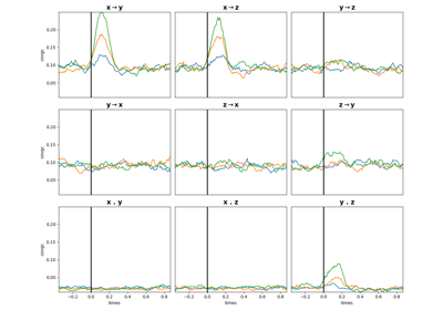
Examples using frites.simulations.StimSpecAR#
AR : conditional covariance based Granger Causality
PID: Decomposing the information carried by pairs of brain regions
Statistical analysis of a stimulus-specific network